오늘은 algorithm 시리즈의 첫 글로 간단한 overview 및 Computational complexity 에 관해 얘기해보고자 한다. 사실 어제 썼던 글이 날아가서 두 번째로 쓰는 것인데.. 다음부터는 글을 올리기 전에 백업을 만들어 놓아야 겠고.. 이번에는 더 나은 글을 쓰기 위함이었다고 긍정적으로 생각해본다.
Contents
- Algorithm
1-1. Data structure - Computational complexity in data structure
2-1. Space complexity
2-2. Time complexity and memoization
2-3. Asymptotic notations - Summary
1. Algorithm
A set of finite rules or instructions to be followed in calculations or other problem-solving operations.
알고리즘은 어떤 문제를 해결하기 위한 규칙이나 절차의 집합이다. 특히나 요새 알고리즘이라는 단어는 SNS 를 이용하는 우리들에게 익숙하게 다가올 것이며, 그것은 개인이 주로 보는 컨텐츠를 기반으로 연관된 글이나 영상들을 제안한다. 이는 빅데이터 기반의 알고리즘을 사용한 결과라고 할 수 있다.
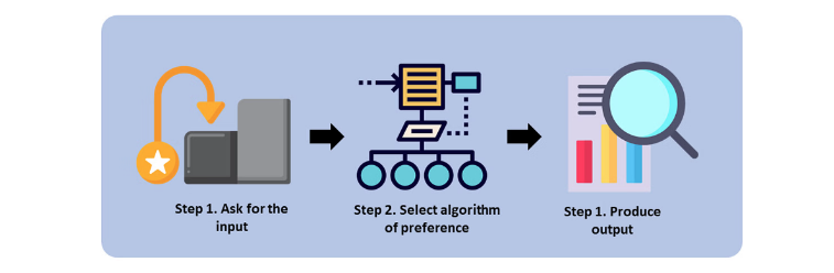
해당 이미지는 알고리즘을 이용한 문제 처리 과정을 보여준다. 데이터 정렬을 예로 들어보자. 우선 1) 컴퓨터는 정렬되지 않은 숫자 리스트를 입력으로 받을 것이고, 2) 가장 적합한 sorting algorithms 를 선택해 정렬을 한 후, 3) 결과적으로 정렬된 숫자 리스트를 출력한다.
따라서, 복잡한 문제를 단계적으로 풀기 위해 알고리즘의 each step 에서는 instruction 이 매우 정확하게 명시되어야한다.
1-1. Data structure
참고로 자료 구조는 데이터의 조직 및 처리 방법 결정에 영향을 미치기 때문에 algorithm 과 밀접한 연관이 있어 간단히 diagram 으로 소개해 보았다.
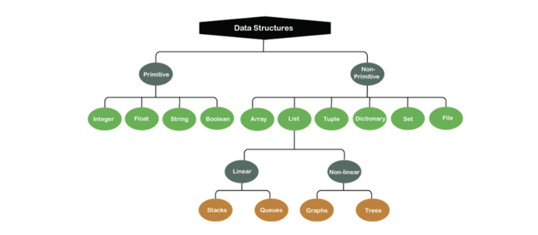
알고리즘에 대해 좀 더 공부하다보면 체감하겠지만, 같은 자료 구조를 쓰더라도 algorithm 의 선택에 따라 코드의 질이 달라질 수 있음을 유의해야 한다.
2. Computational complexity in data structure
그렇다면 우리는 과연 좋은 알고리즘을 선택했는지 어떻게 알 수 있을까? 이 질문에 대한 답으로 computational complexity (space and time complexity) 를 들 수 있다.
An algorithm's complexity is a measure of the amount of data it must process to be efficient.
우리는 daily tasks 를 해결함에 있어 가장 효율적인 방법을 모색한다. 이는 컴퓨터 또한 마찬가지이다. 최선의 작동을 위해 우리는 time efficient 하고 less memory 를 필요로 하는 알고리즘을 개발 및 사용해야 할 것이다.
2-1. Space complexity
먼저 공간 복잡도 또는 space complexity 는 어떤 프로그램을 실행 및 완료하는데 필요한 메모리 공간의 양이다. 단, 현대에는 컴퓨터 저장공간 기술의 발달로 시간 복잡도에 비해 공간 복잡도의 중요성은 낮아졌다.
The amount of memory used by a program to execute the code is represented by its space complexity.
이 때, 프로그램이 요구하는 메모리는 다음의 수식처럼 input space (고정 공간, c) 와 auxiliary space (가변 공간, S_p(n)) 의 합으로 표현된다.

- Input space - 알고리즘과 관계 없는 코드 저장 공간
A memory space used by its inputs (variables, constants, ..).- Auxiliary space - 알고리즘 실행 중 동적으로 필요한 공간
An extra or temporary space used by an algorithm during execution.
2-2. Time complexity and memoization
그 다음으로 시간 복잡도 또는 time complexity 는 특정 알고리즘이 어떤 문제를 해결하는데 걸리는 시간이다.
Time complexity represents the time it takes to run or solve a given algorithm.
단, 시간 복잡도가 예측하는 것은 전체 execution time 이 아니라 문제 해결 시 성능 또는 시간에 많은 영향을 주는 연산량 따위의 부분에 대한 시간이다. 예로 들자면 반복문의 연산량이 있을 것이다.
참고로 만약 massive 한 연산량 때문에 문제 해결 시간이 상당히 길어진다면 memoization 을 이용하자. 이는 메모리를 더 많이 사용해 시간을 비약적으로 줄이는 optimization technique 으로서, 시간 복잡도와 공간 복잡도 사이의 거래 관계 (aka space-time tradeoff) 가 성립함을 이용하였다.
2-3. Asymptotic notations
그렇다면 space 와 time complexity 를 비교하기 위해 asymptotic analysis 를 적용해보자.
Asymptotic notations are programming languages that allow you to analyze the algorithm's running time by identifying its behavior as its input size grows (i.e., the algorithm's growth rate).
- 참고 링크: Asymptotic notations 에 관한 간단한 설명을 제공한다.
https://www.boardinfinity.com/blog/asymptotic-analysis/
다음은 세 가지의 asymptotic notations 를 나타낸 그래프들이다. x-axis 는 input size 그리고 y-axis 는 operation time or steps 라고 보면 되겠다.
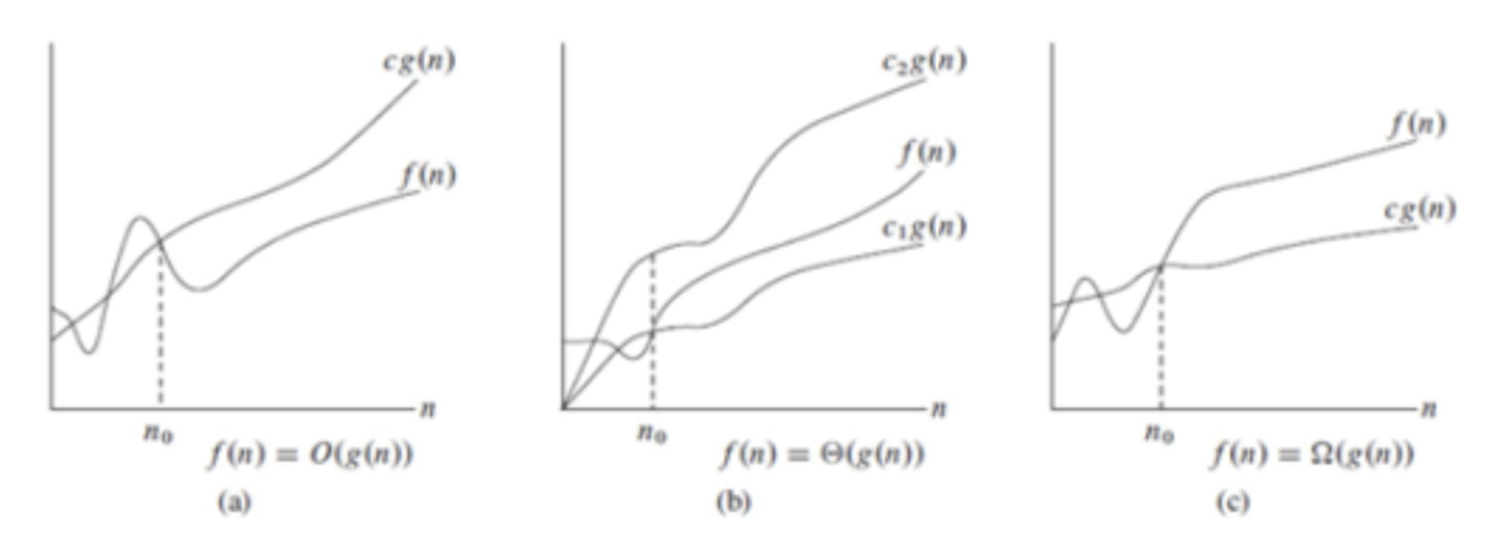
(a) Big-O (worst case)
The asymptotic upper bound of a running time of an algorithm with the most time required.
Big-O notation 은 최악의 경우로서 가장 긴 runtime 을 필요로 한다. 따라서 Big-O 는 주로 huge input 을 가진 알고리즘에 대해 worst-case time complexity 를 찾는데 도움이 된다.
(b) Big-Θ (average case)
The tight bound of a running time with the average time required.
(c) Big-Ω (best case)
The lower bound of a runtime algorithm that gives the best-case time complexity.
Big-O 와는 반대로 Big-Ω 는 최선의 경우를 나타내어 가장 짧은 runtime 을 요구한다.
3. Summary
여기까지 간단히 알고리즘에 대한 소개와 complexity 에 대해 알아보았다. 이 때, time complexity 에 관하여 특정 알고리즘 외에는 주로 Big-O 를 사용하기 때문에 다음 글에서는 Big-O 에 대해 조금 더 자세히 다루어보려 한다.
