Algorithm (2) - Big-O notations, sorting algorithms

이전 글에서는 space 와 time 으로 나뉘는 computational complexity 에 관해 알아보았다면, 이번에는 그 중 더욱 중요시 되는 time complexity 의 Big-O notations 을 조금 더 자세히 다루어보겠다.

Contents

1. Big-O notations
   1-1. $O(1)$
   1-2. $O(log n)$
   1-3. $O(n)$
   1-4. $O(n・log n)$
   1-5. $O(n^2)$
   1-6. $O(c^n), c>1$

---

1. Big-O notations

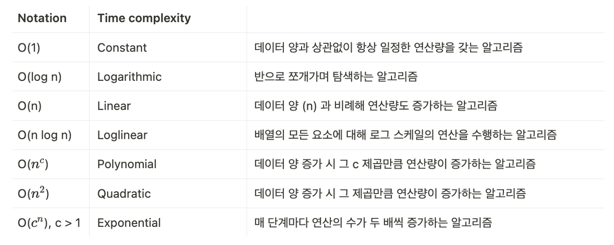
다음은 알고리즘의 runtime 을 분석하기 위해 흔히 사용되는 함수들을 요약해 놓은 표이다. 아래로 내려갈수록 complexity 는 더 증가한다. 이전에도 언급했듯이 time complexity 는 알고리즘의 performance 와 efficiency 를 평가하기 위해 사용되고, 특히 Big-O 는 worst-case time performance 를 확인하기에 유용하다.

즉, 원소의 개수 (n 개) 에 대한 알고리즘을 실행하기 위해 필요한 단계의 수를 나타내기 위해 Big-O 를 사용하게 되었다.

---

1-1. Constant complexity: $O(1)$

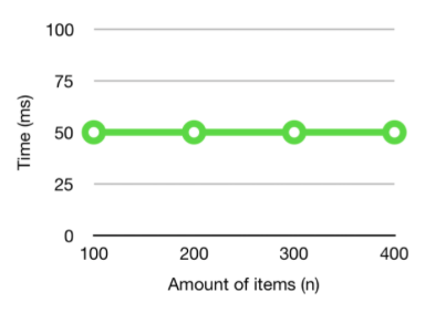
The algorithm will run in the same amount of time, no matter the input size (n).

알고리즘이 상수 복잡도를 갖는다면 항상 operation time 이 일정하다. 예를 들어 어떤 array 의 첫 번째 element 를 찾으려 한다면, input size 에 상관없이 array[0] 을 이용하여 해결할 수 있기 때문에 runtime 의 변함이 없다.

---

1-2. Logarithmic complexity: $O(log n)$

The size of the input we are considering gets split into half with each iteration.

로그 복잡도에서의 log n 은 base 가 2 인 것이 생략된 것이다. 따라서, 해당 알고리즘에 어떠한 입력값 n 개가 들어왔다면 매번 반으로 나누어지며 탐색하게 된다. 예를 들어 input size (n) = 8 을 execute 할 때 3초가 걸렸다고 해보자. 그렇다면 n= 16 는 그것의 4초가 걸릴 것이고, n = 32 는 5초가 걸린다.

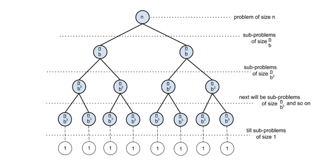
로그 복잡도의 예로는 sorted array 에서 binary tree 를 이용한 특정 원소를 찾기를 들 수 있다. Binary tree 는 n 개의 원소가 size 가 1이 될 때까지 n/2 의 subgroups 로 나뉜다. 그러므로 위의 tree 를 resolve 하기 위해 필요한 operations 는 O(log n) 이 된다.

---

1-3. Linear complexity: $O(n)$

The runtime of an algorithm grows almost linearly with the input size.

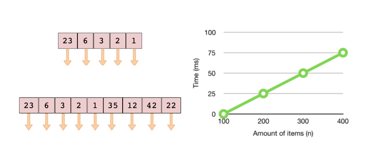
간단히 말해 선형 복잡도는 데이터의 양 (n) 만큼 operation 도 증가하는 linear graph 를 그린다. 이것의 예들로는 array 전체를 looping 또는 탐색해야 하는 문제들이 있다. Unsorted array 에서 특정 원소를 찾는 알고리즘 가정해보자.

for i in range(n):
  sum_ += 1

이 때, array 의 원소가 많으면 많을수록 전체 원소를 looping 하는 시간이 길어지게 된다. 각 요소들을 invoke 하기 위해 5 ms 가 걸린다고 한다면 아래처럼 5 개의 원소에 대해서는 총 25 ms, 그리고 9 개의 원소에 대해서는 총 45 ms 가 소요된다.

• 참고 링크: $O(1), O(log n), O(n)$ 의 비교 및 Big-O 표기법 연습 문제를 제공한다.
  https://velog.io/@on-n-on-turtle/누구나-자료구조와-알고리즘-빅오-표기법이-필요한-이유

---

1-4. Loglinear complexity: $O(n・log n)$

The algorithm applies $log n$ operations $n$ times to every element in an array.

다양한 logarithmic complexities 중에는 n・log n 의 선형 로그 복잡도 또한 존재하는데, loglinear complexity 는 주로 Quick sort, Merge sort, Heap sort 와 같은 recursive sorting algorithms 또는 binary tree sorting algorithms 에 사용된다. 다음의 merge sort 가 작동하는 원리를 참고해보자.

Here $n$ is the size of data structure (array) to be sorted and $log n$ is the average number of comparisons needed to place a value at its right place in the sorted array.

---

1-5. Quadratic complexity: $O(n^2)$

The runtime scales quadratically with the input size ($n$). That is, the runtime is proportional to the squre of the input size.

Polynomial 중에서도 quadratic complexity 는 데이터의 양 (n) 이 증가함에 따라 그 제곱만큼 operation 이 증가한다. 예를 들어, input size 가 n = 1 일 때는 1 step 이, n = 10 일 때는 100 steps 가, n = 100 일 때는 10,000 steps 가 걸린다.

A common example is by looping over an array and comparing the current element with all other elements in the array.

2차 복잡도에 해당하는 sorting algorithms 로는 다음의 bubble sort 나 insertion sort 등이 있다.

def bubble_sort(arr):
    n = len(arr)
    
    for i in range(n):
        for j in range(n-i-1):
            if arr[j] > arr[j + 1]:
                arr[j], arr[j + 1] = arr[j + 1], arr[j]


print(bubble_sort([5, 4, 3, 2, 1]))

위의 코드를 참고하면, 우리는 총 n 개의 요소들을 검사하는 동안 또 다시 다른 n 개의 요소들과 비교와 정렬을 하게 된다. 따라서, $n^2$ 만큼 연산을 하는 것이다.

---

1-6. Exponential time: $O(c^n), c>1$

For $O(2^n)$, the runtime is doubled with each additional input element.

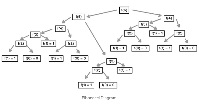
마지막으로는 지수 복잡도가 있다. Base 가 c = 2 인 exponential time 에 대하여, 만약 5 개의 원소에 대한 연산을 하는데 30초가 걸렸다면 6 개의 원소에 대해서는 그 시간의 2 배인 60초가 걸림을 알 수 있다. 이것의 대표적인 예시로는 recursive fibonacci sequence 가 있다.

• 참고 링크: 피보나치 수열의 recursive method 에 대해 자세한 설명이 제공된다.
  https://medium.com/launch-school/recursive-fibonnaci-method-explained-d82215c5498e