🔎 Stanford CS231n 강의를 듣고 기록용도로 정리하는 게시글입니다.

Neural Network

"Vanilla" Neural Network

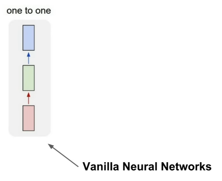
• so far, we saw a vanilla feed forward network
  • receive input, which is a fixed size object(ex. image, vector..)
  • input is fed through set of hidden layers
  • produces a single output (ex. a set of classifications scores over a set of categories)

Recurrent Neural Network: Process Sequences

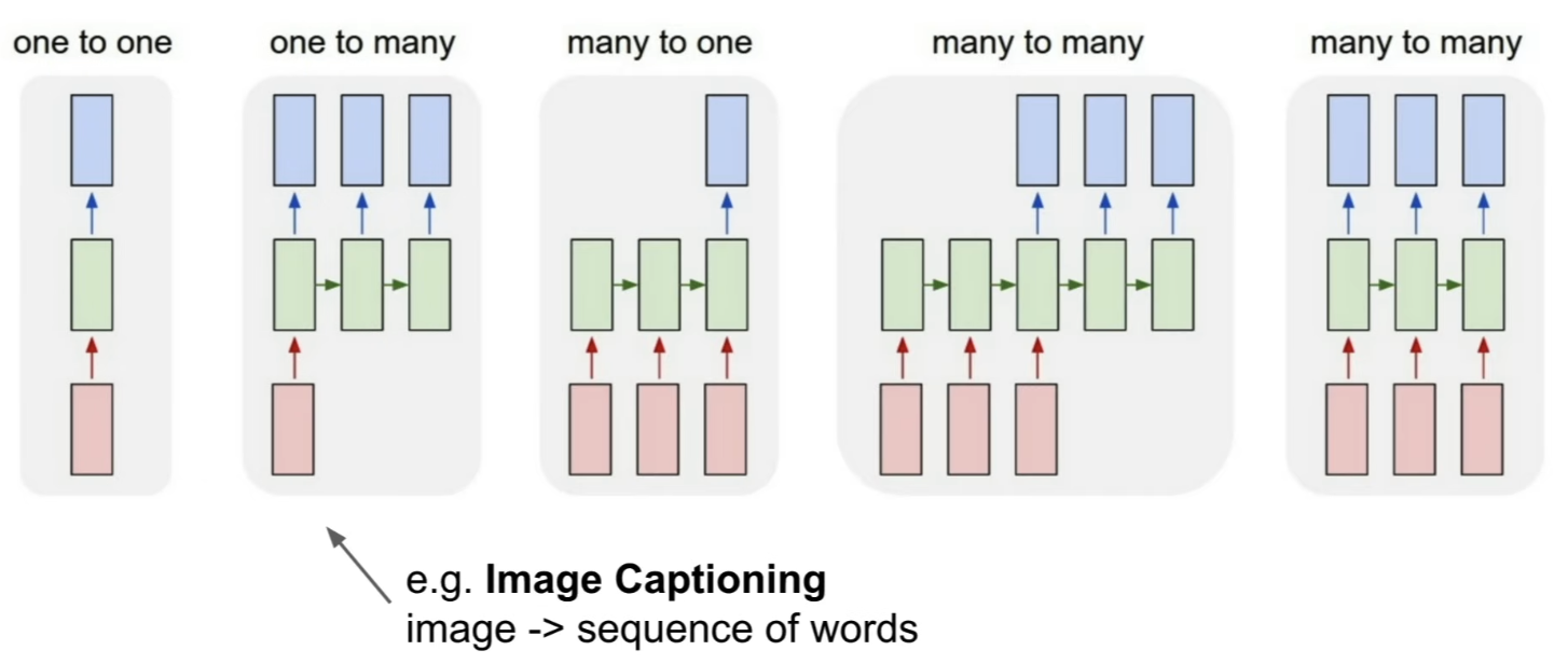
• but in ML, we want to have more flexibility in the types of data that our model can process
• in Recurrent Neural Network, we have a lot more opportunities with types of input and output data that our networks can handle
  • with this, we can do one-to-many models; input is some object of fixed size (ex.image), but output is a sequence of variable length(ex.caption)
  • many-to-one model: input could be variably sized(ex.piece of text), and say what the sentiment of that text is (positive or negative)
    • in CV context, input as a video(=variable number of frames), make a classfication decision of what kind of activity or action is going on in that video
  • many-to-many model: both the input and output to be variable in length (ex. machine translation)
  • many-to-many model: input is variably length(ex. video sequence with a variable number of frames), want to make a decision for each element of that input sequence
    • in the context of videos, this might be making decision along every frame of the video

Sequential Processing of Non-Sequence Data

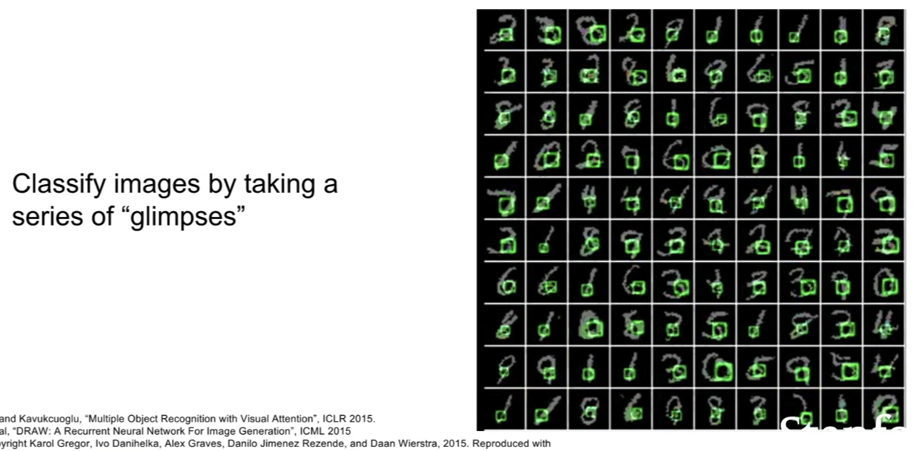
• receiving a fixed size input (image)
• want to make a classification decision about what number is being shown in the image
• rather than doing a single feed forward pass and making the decision all at once,
  • this network is looking around the image and taking various glimpses of different parts of the image
  • after making some series of "glimpses", makes final decision

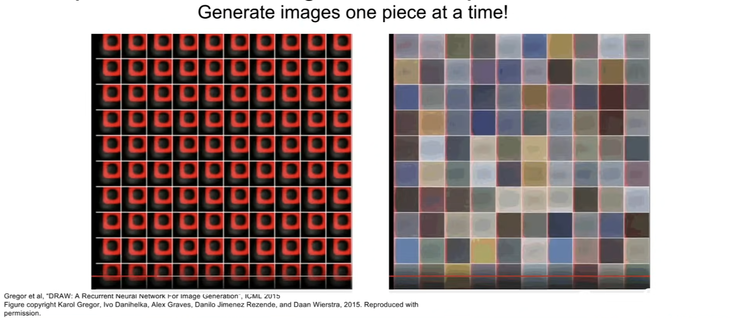
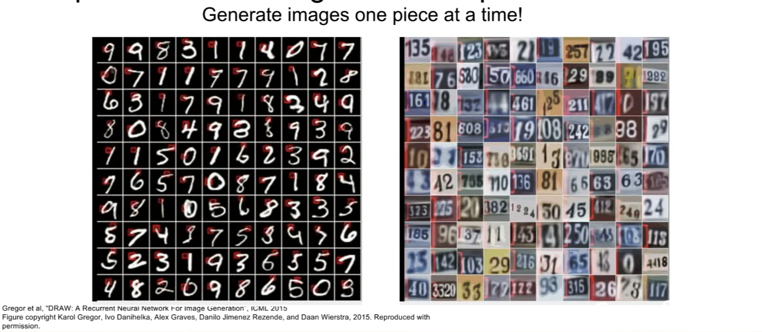
• now we want the model to synthesize brand new images that look like the image it was in training, we can use a recurrent neural network architecture to paint these output images one piece at a time in the output
  • even though output is a fixed size image,
  • we can have models that are working over time to compute parts of the output one at a time sequentially

Recurrent Neural Network

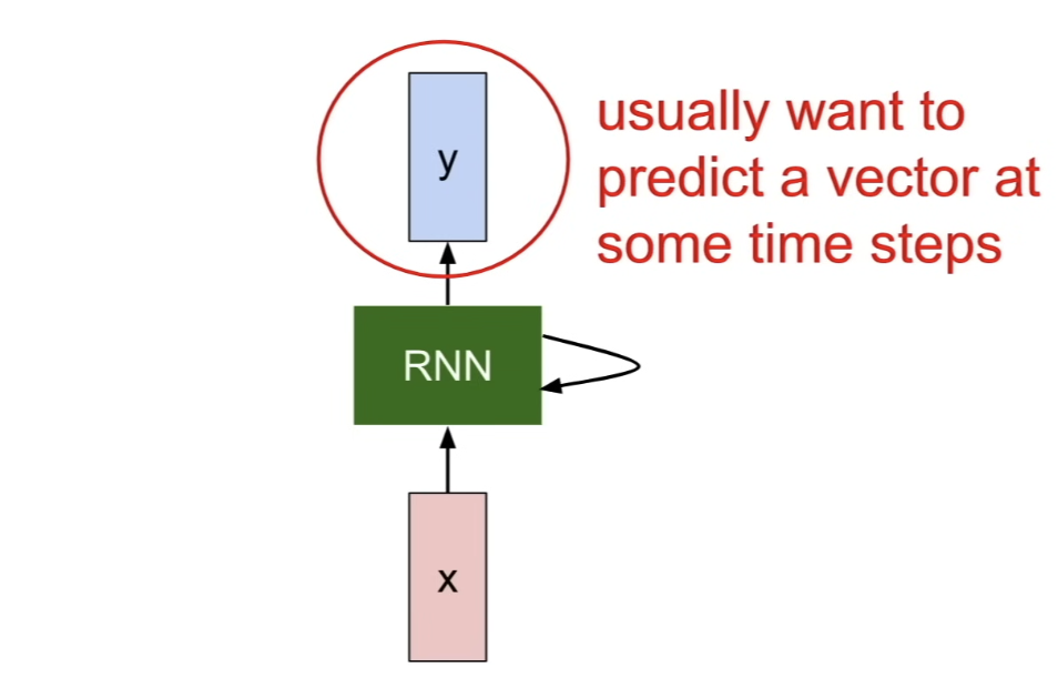
• overview of RNN

  • there is a recurrent core cell that takes some input $x$ and feed that input into the RNN
  • that RNN has some internal hidden state and that hidden state will be updated everytime the RNN reads a new input
  • then, the internal hidden state will be fed back to the model the next time it reads an input

• we want our RNNs to produce some output at every time step

  • a pattern where it reads an input → update its hidden state → produces output

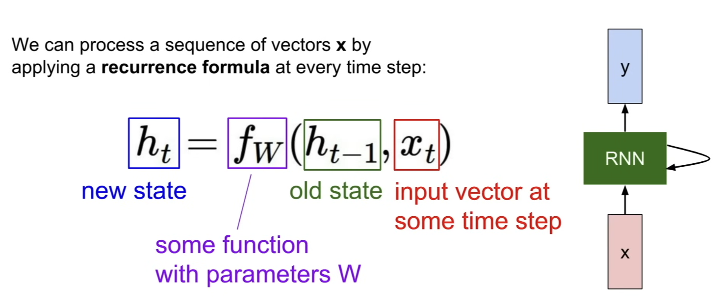
• What is the functional form of this recurrence relation that we're computing?
• Inside the RNN block, we're computing some recurrent relation, with a function $f$
  • $f$ will depend on some weights $W$
  • $f$ will accept the previous hidden state, $h_{t-1}$, as well as the input at the current state $x_t$
  • $f$ outputs the next hidden state, or the updated hidden state, $h_t$
• If we want to produce some output at every time step, might attach some additional fully connected layers that read in $h_t$ at every time step
  • make that decision based on the hidden state at every time step
• Notice: the same function and the same set of parameters are used at every time step

Vanilla RNN

• simplest functional form
  
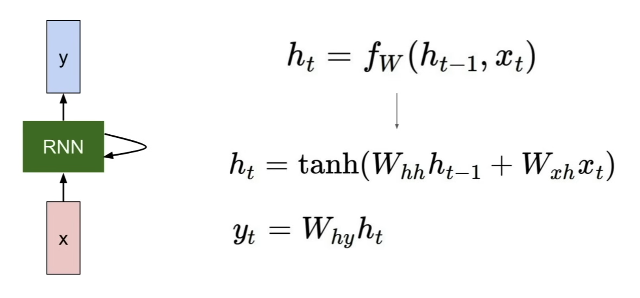
• make 2 multiplications against 2 states → add them → squash them using $\tanh$, so we get some non-linearity in the system
• in addition, if we want to produce some $y_t$ at every time step, we need another weight matrix $W_{hy}$ that accepts this hidden state and transforms it to some $y$ to produce maybe class score predictions

RNN: Computational Graph

• you can think of RNN in 2 ways
  • concept of having a hidden state that feeds back at itself, recurrently
  • unrolling this computational graph for multiple time steps

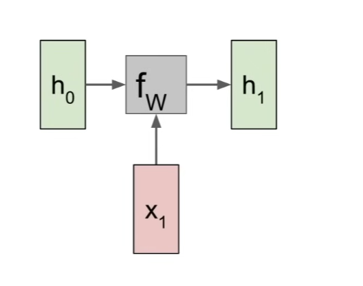
• initial hidden state, $h_0$ (initialized to 0 in most contexts)
• input $x_1$
• $h_0$ and $x_1$ will go into $f_w$ function, and produce next hidden state, $h_1$

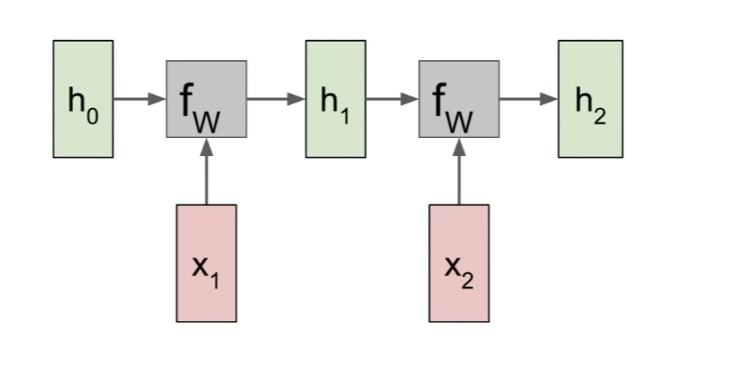
• repeat this process when we receive the next input
• current $h_1$ and $x_2$ will produce next output, $h_2$

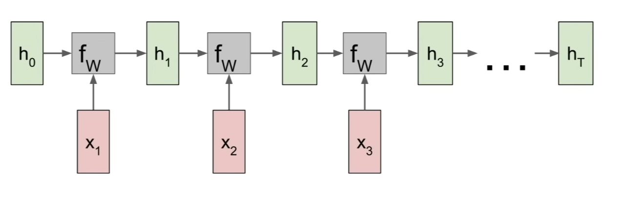
• repeat this process over and over again, as we consume all of the input, $x_t$s, in our sequence of inputs

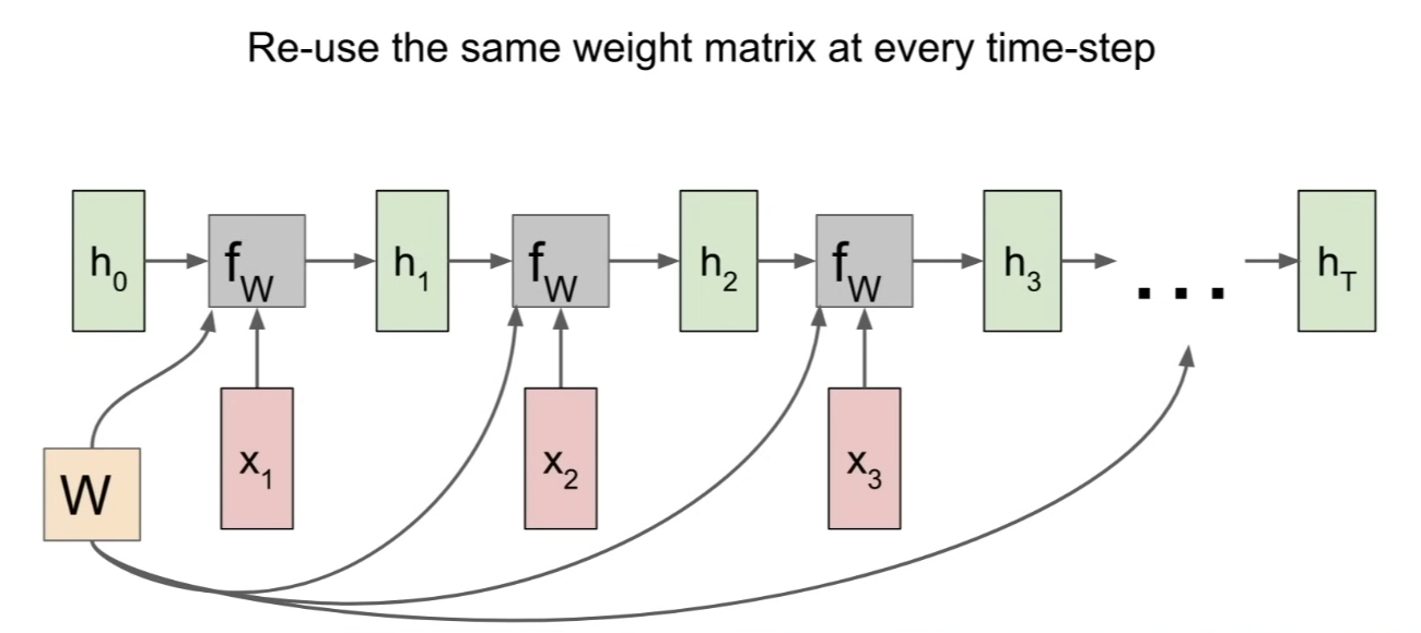
• we can make this more explicit and with $W$ matrix in computational graph
  • we're re-using the same $W$ matrix at every time step of the computation
  • all of the $f_W$ blocks are taking unique $h$ and unique $x$, but same $W$
• when re-using the same node multiple times in a computational graph, during backward pass, you end up summing the gradients into the $W$ matrix when computing $dW$
  • backpropagation for this model: get a separate gradient for $W$ flowing from each of the time steps, and the final gradient of $W$ will be the sum of all of those individual per time step gradients

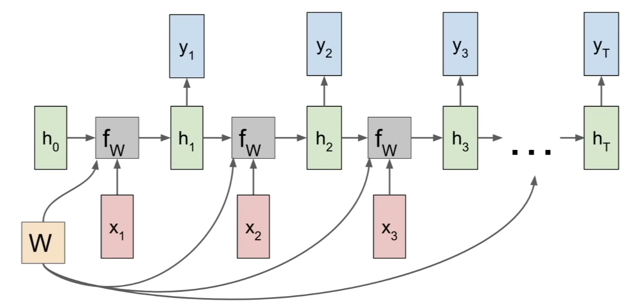
• we can write $y_t$ explicitly
  • output $h_t$ at every time step, might feed into some other little neural network that can produce $y_t$, which might be some class scores

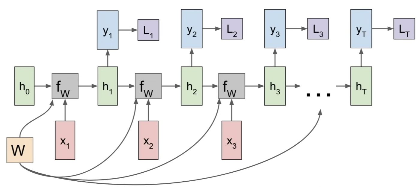
• we can make the $Loss$ more explicit
  • imagine having ground truth label at every time step of the sequence
  • and you'll compute some individual loss at every time step of outputs, $y_t$s
    • the loss will frequently be something like Softmax loss
  • final loss = sum of individual losses
  • backpropagation - in order to train the model, we need to compute gradient of the loss with respect to $W$
    • so, we'll have the final loss flowing into each of these time steps
    • at each time step, compute a local gradient on the weights $W$
      ⇒ these will be summed to give us the final gradient for the weights $W$
      

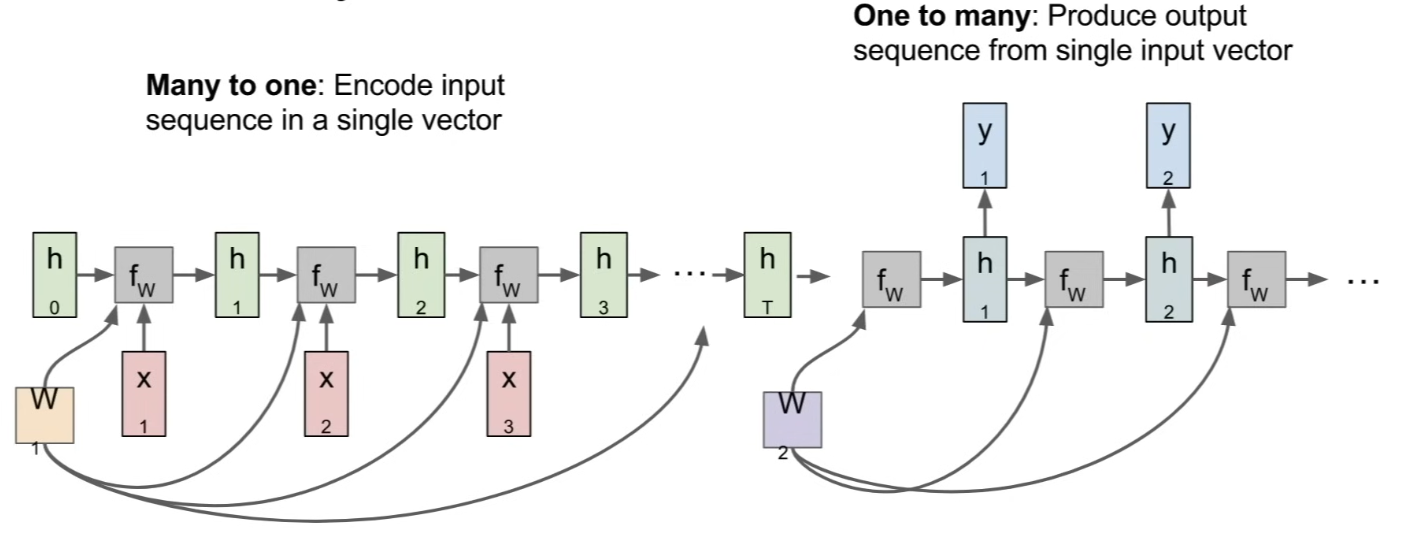
Many-to-One

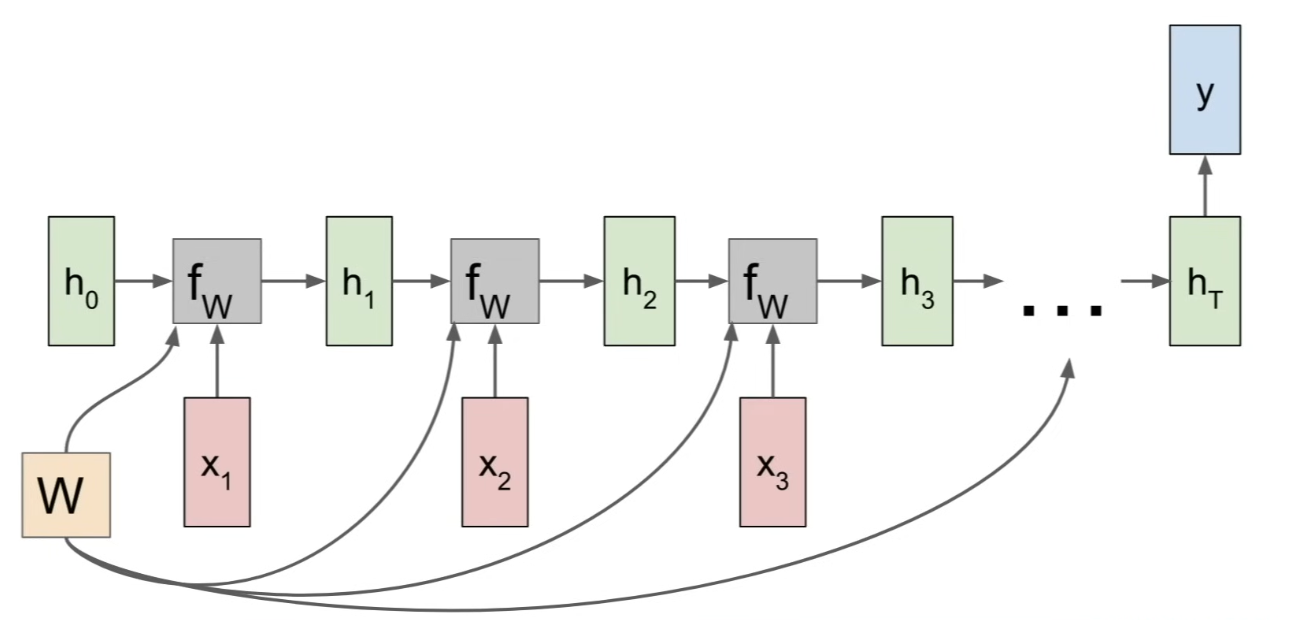
• typically make a decision based on the final hidden state
  • b/c final hidden state summarizes all of the context from the entire sequence

One-to-Many

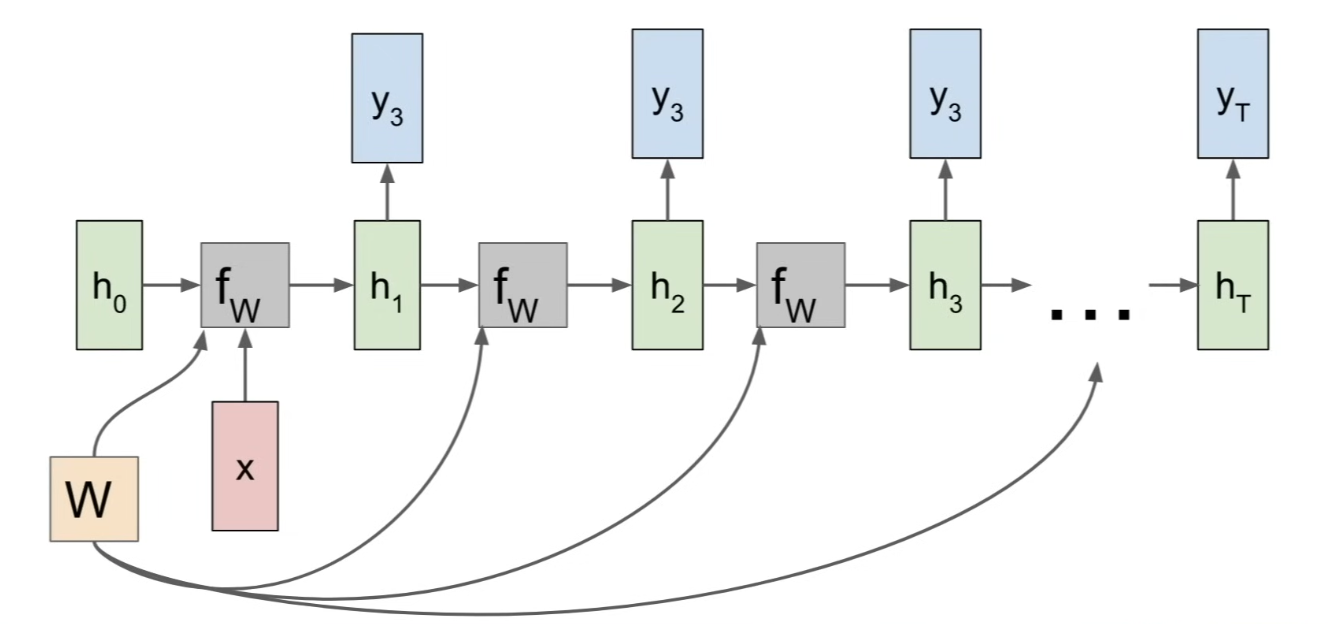
• receiving a fixed size input and produce a variably sized output
• use the fixed size input to somehow initialize the initial hidden state of the model
• as you produce variably sized output, you'll unroll the graph for each element in the output

Many-to-Many (Sequence to Sequence)

• ex) machine translation

• take a variably sized input, and produce a variably sized output
  

• think of it as a combination of many-to-one + one-to-many

  • 2 stages; encoder and a decoder
    • encoder: receive variably sized input (ex. sentence in English) → summarize the entire sentence using the final hidden state of the encoder network
    • decoder: input the single vector (summarized input sentence) and produce variably sized output(sentence in another language) (at every time step, we might make some predictions about what word to use)

• train this entire thing by unrolling this computational graph, summing the losses at the output sequence, and performing backpropagation

Language Modeling problem

• we want the network to understand how to produce natural language
• producing might happen at..
  • character level; produce character one at a time
  • word level; produce words one at a time
• simple example: character level language model
  • read some sequence of characters and needs to predict what the next character in this stream of text will be

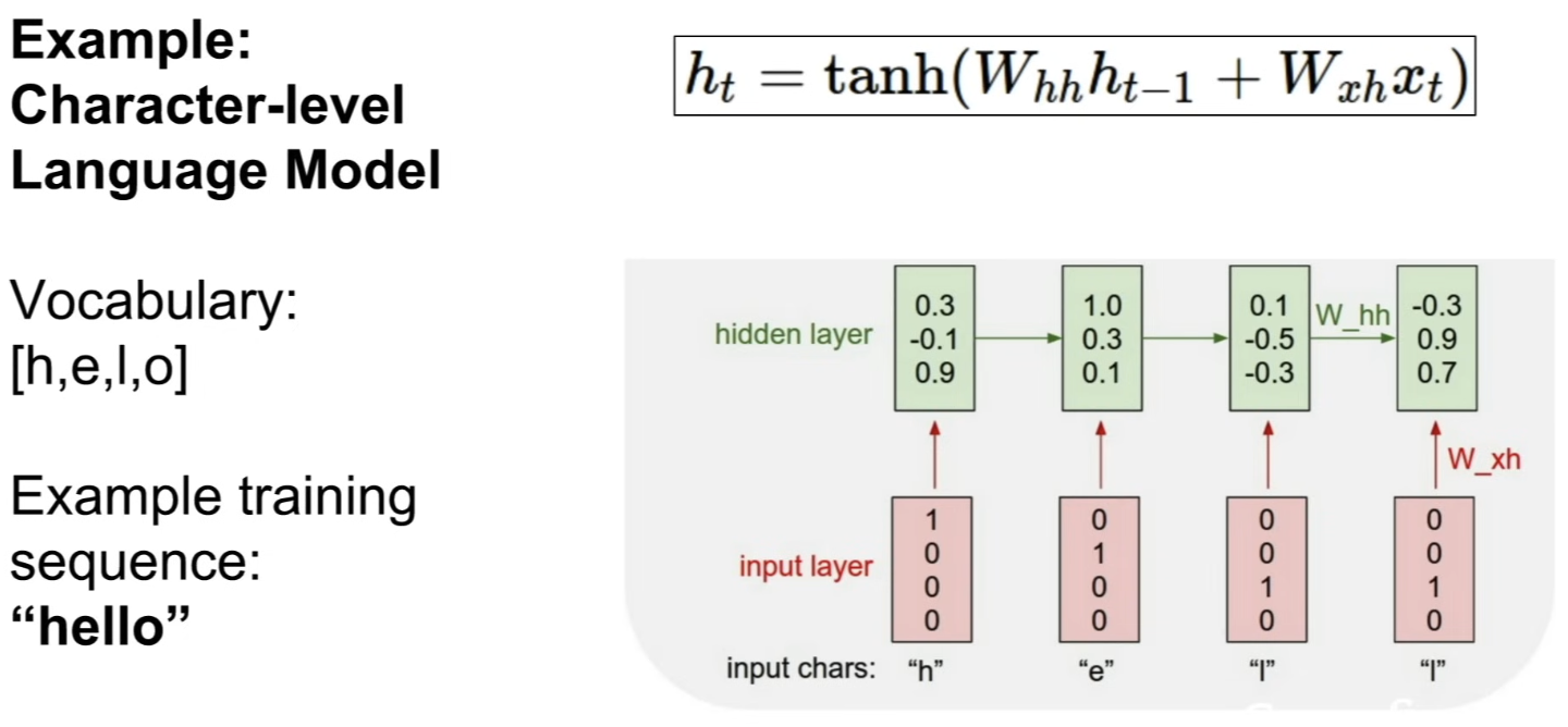
• when training, feed the characters of this training sequence as inputs, $x_t$s, to our recurrent neural network
• each of these inputs are letters → we need to figure out a way to represent letters in our network
  • so, figure out what our total vocabulary is
  • in this case, we have 4 elements in our vocabulary, and each letter will be represented by a vector that has 0s in every slot but 1, for the slot in the vocabulary corresponding to that letter

Forward pass

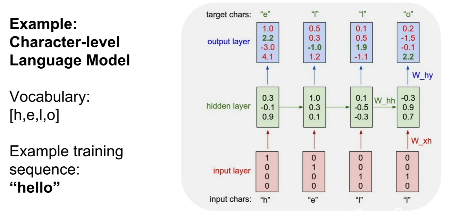
• 1st time step: receive input letter 'h' → go into the 1st RNN cell → produce $y_t$, which is the network making predictions for each letter in the vocabulary, about which letter is likely to be going to come next

  • it's actually predicting 'o' as the most likely letter → wrong, use softmax loss to quantify our unhappiness with these predictions

• next time step: feed in the 2nd letter in the training sequence, 'e' → repeat the process

  • represent 'e' as a vector → use that input vector together with the previous hidden state to produce a new hidden state
  • use the 2nd hidden state again, to make predictions over every letter in the vocabulary

• if you train this model with many different sequences, it should eventually learn how to predict the next character in a sequence based on the context of the previous characters that it's seen before

Test time

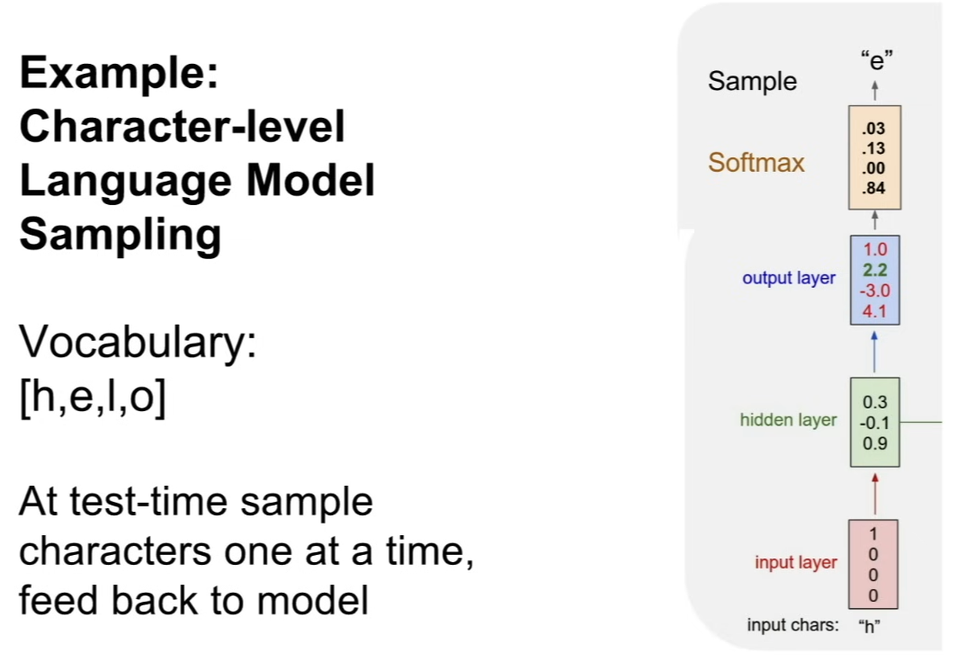
• after training, we might want to sample from the model, and use this trained neural network model to synthesize new text that looks similar to the text that it was trained on
  • see the model with some input prefix of text
    • in this case, prefix is a single letter 'h'
  • feed the letter 'h' through the 1st time step of the RNN
  • produces distribution of scores over all the characters in the vocabulary
• in the test time, we'll use these scores to actually sample from it
  • use a Softmax function to convert the scores into a probability distribution
  • then, sample from that probability distribution to actually synthesize the 2nd letter in that sequence
  • take the letter 'e' that was sampled from this distribution, feed it back as input into the network at the next time step

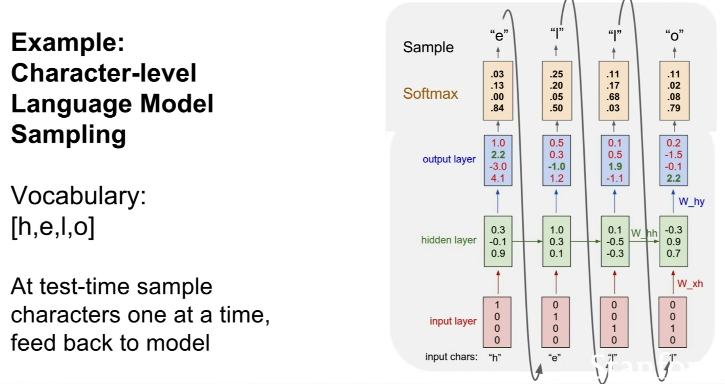
• repeat this process over and over again to synthesize a new sequence using this trained model
  • synthesizing the sequence 1 character at a time, using these predicted probability distributions

Q: Why sample instead of taking the character with the largest score?
A: b/c of the probability distribution that we had, it was impossible to get the right character, so we had to sample so the example could work out.. but in practice you'll see both

Backpropagation through time

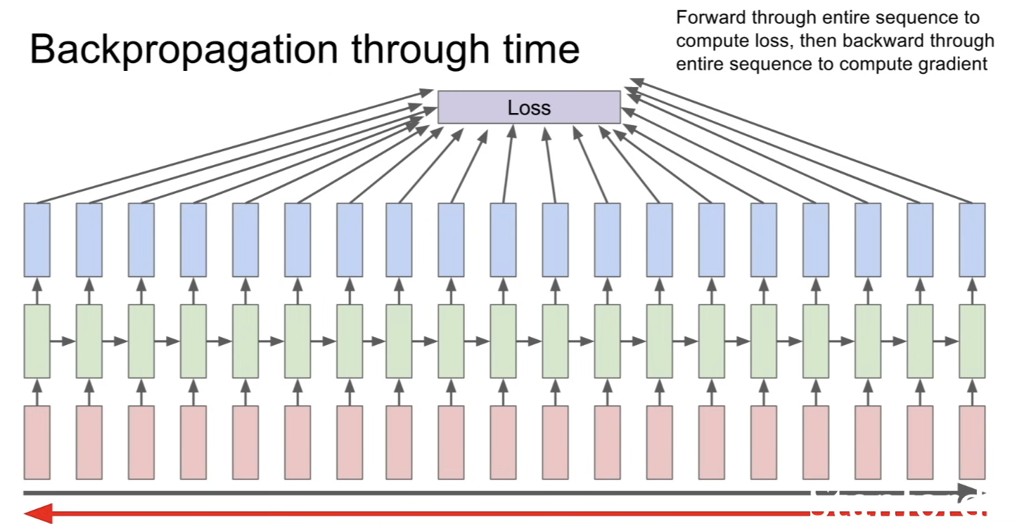
• having a sequence, produce output at every time step of the sequence, and computing some loss = Backpropagation through time
  • forward pass - stepping forward through time
  • backward pass - going backwards through time to compute gradients
• this is problematic when you want to train the sequences that are very long
  • ex) training RNN on the entire text of Wikipedia → super slow → every time we make gradient step, we would have to make a forward pass through the entire text of all of wikipedia, and make a backward pass through all of wikipedia, and then make a single gradient update
    • will be super slow, model will never converge, will take a ridiculous amount of memory

Truncated Backpropagation through time

• in practice, we do some approximation called Truncated(생략된) Backpropagation through time
  
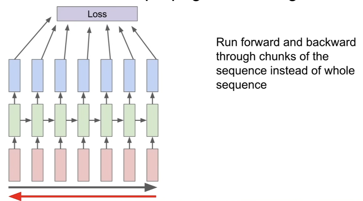
• even though the input sequence is very long, when training,
  • we'll step forward for some number of steps(ex.100)
  • compute a loss only over this subsequence of the data,
  • then backpropagate through this subsequence
  • make a gradient step

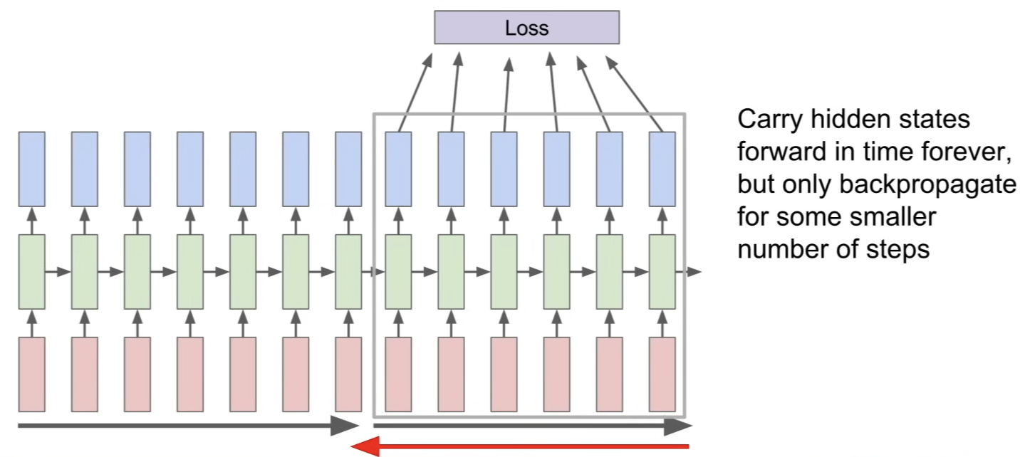
• when we repeat, we still have these hidden states that we computed from the 1st batch
• when we compute the next batch of data, we will carry those hidden states forward in time
  • when computing a gradient step for this next batch of data, only backpropagate again through this 2nd batch
  • and make a gradient step based on this truncated backpropagation through time

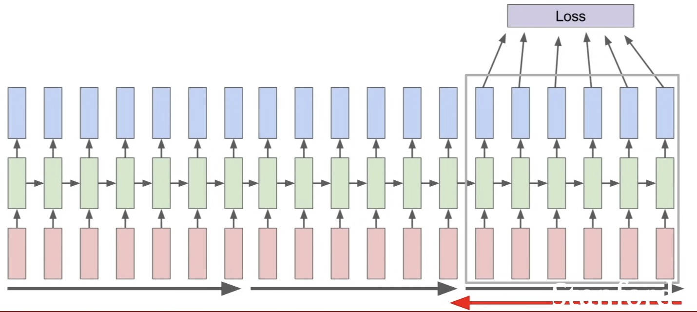
• repeat the process
• step forward and backward only for some small number of time steps

Searching for interpretable cells

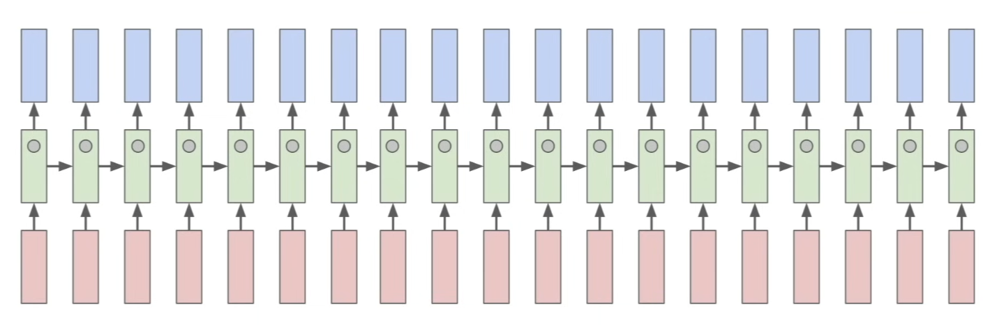
• figuring out what the model is doing and why they are working?
  • these RNNs have these hidden vector which is some vector that gets updated over time
• Could we find some elements of this vector that have some semantic interpretable meaning?
  ⇒ trained a neural network language model, picked one of the elements in that hidden vector and look at the value of that hidden vector over the course of a sequence, to try to get some sense of what these different hidden states are looking for

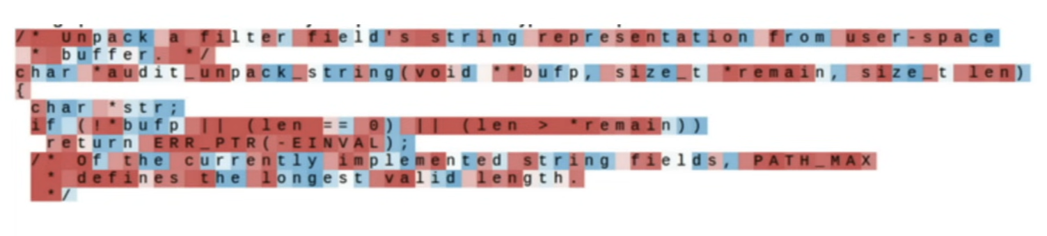
• picked 1 element of that vector, and run the sequence forward through the trained model
• color of each character corresponds to the magnitude of that single scalar element of the hidden vector at every time step
• a lot of the vectors in these hidden states are not very interpretable
  • seems like it's doing low level language modeling to figure out what character should come next

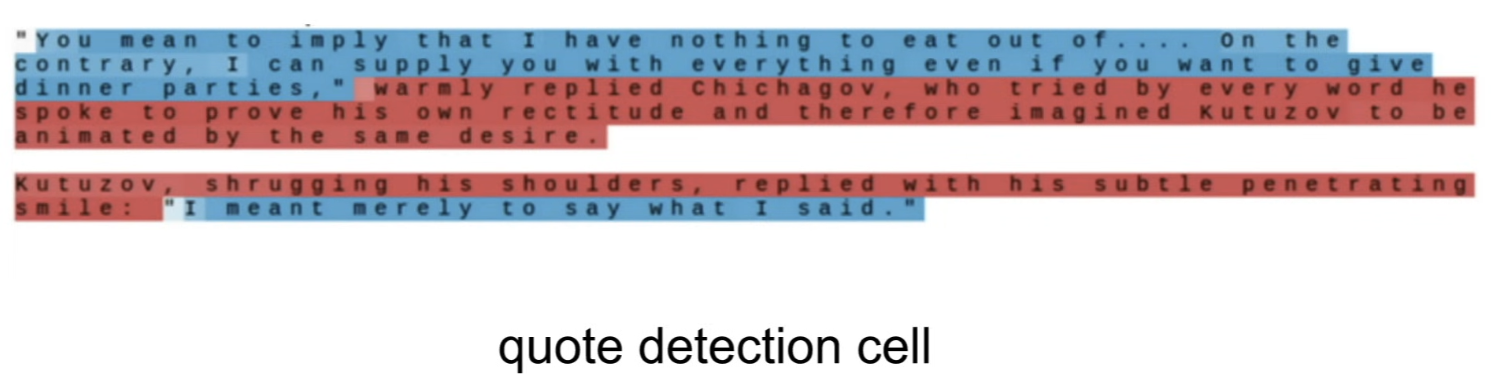
• But, some of them ended up quite nice
• here is the vector that's looking for quotes
  • this 1 element in that vector; once it hits the quote, it turns on and remains on for the duration of this quote
  • when we hit the 2nd quotation mark, cell turns off

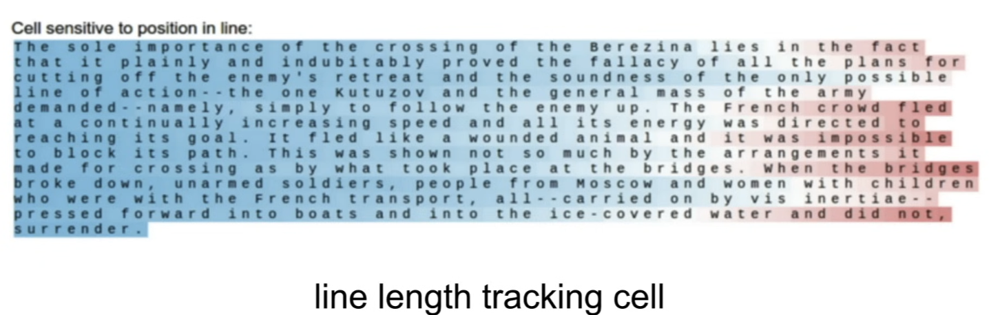
• cell that looks like it's counting the numbers of characters since a line break
• at the beginning of each line, this element starts off at 0 → throughout the course of the line, it gets gradually more red = value increases
• this cell is letting the network keep track of when it needs to produce new line characters

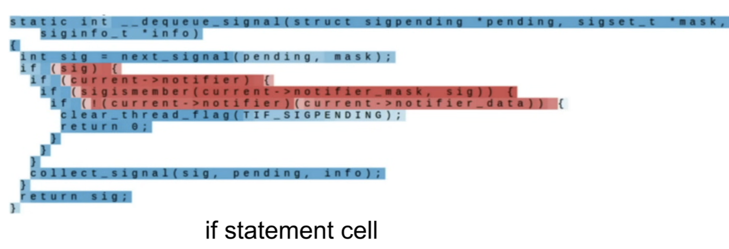
• trained on the linux source code,
  • cells turning on inside the conditions of if statements
• this maybe allows the network to differentiate whether it's outside an if statement or inside that condition → help it model these sequences better

Image Captioning

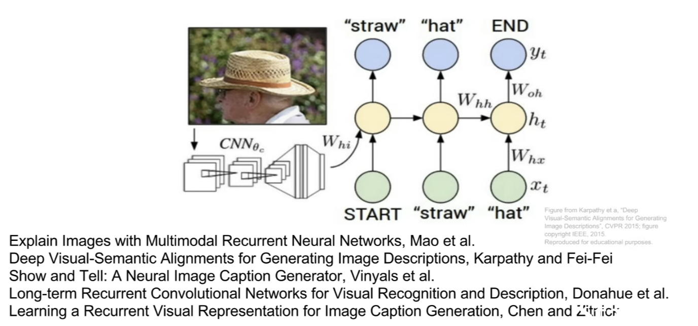
• image captioning model: input an image, output a caption in natural language
• caption: variable length sequence ⇒ totally natural fit for a RNN model

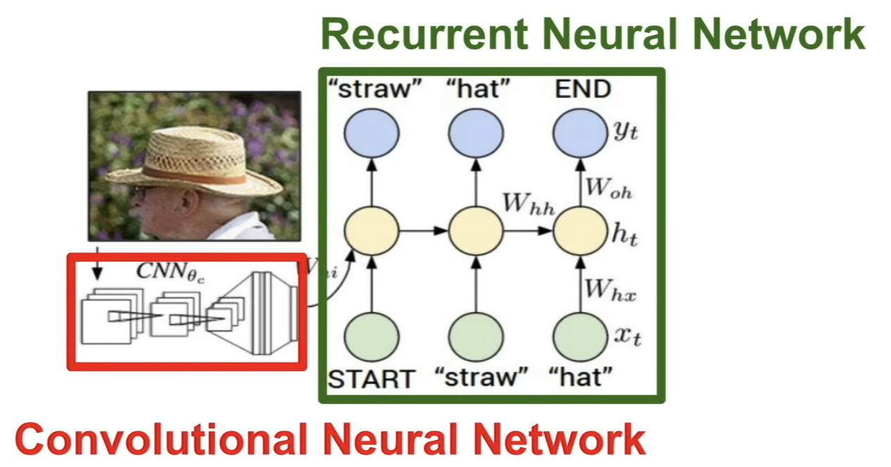
• ConvNet: take an image as the input, produce a summary vector of the image, which will feed into the first time step of RNN
• RNN: produce words of the caption one at a time

Test time

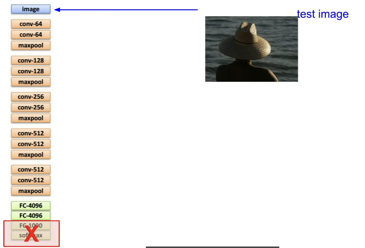
• take input image, feed it through ConvNet
  • instead of taking the Softmax scores from an ImageNet model, take the 4096 dimensional vector from the end of the model
  • take the 4096-dimensional vector to summarize the whole content of the image
• in RNN, we need to see the language model with that first initial input to tell it to start generating text (→ prefix?)
  • so in this case, give it some special start token, which says that this is the start of a sentence

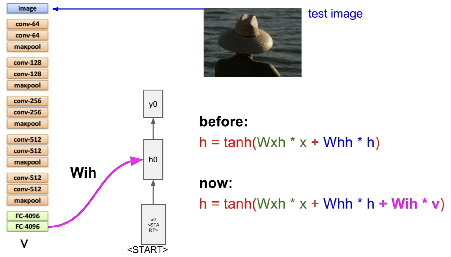
• previously, we saw that RNN model has 2 matrices that were taking the input at the current step and the hidden state of the previous time step, and combining those to get the next hidden state
• But now, we also need to add this image information(4096-dimensional vector ..thing)
  • one simple way is to add a third weight matrix that is adding in this image information at every time step

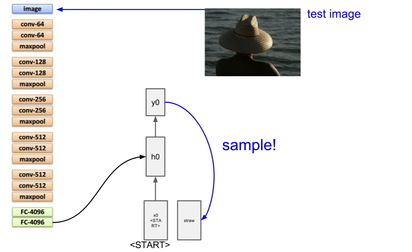
• now, we'll compute the distribution over all scores in our vocabulary(here, the vocabulary is all English words)
• sample from that distribution → pass that word back as the input for the next time step
  
  
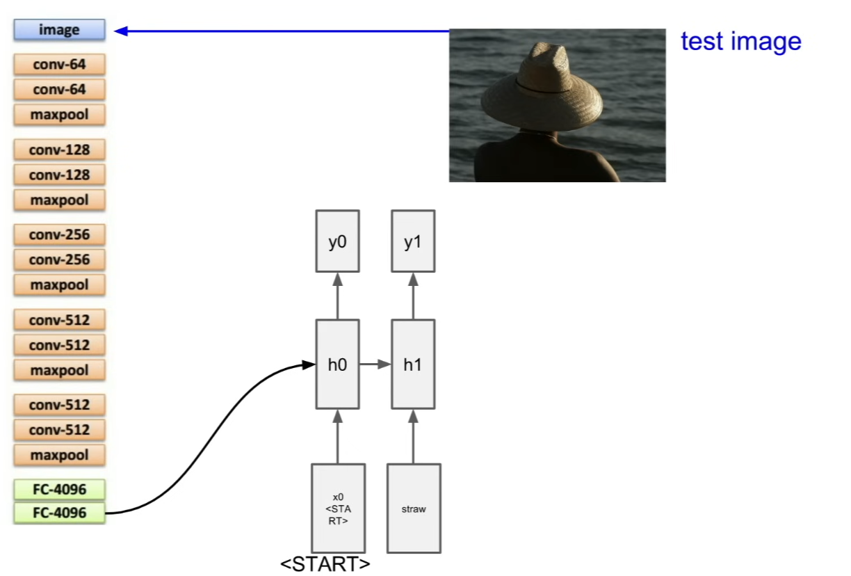
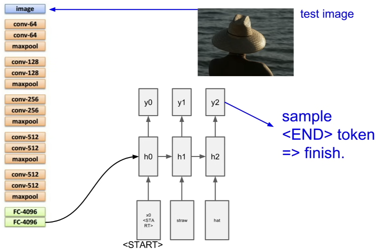
• after everything is done, we'll generate this complete sentence
• we stop generation once we sample the special ends token, which corresponds to the period at the end of the sentence
  • during training, we put an end token of every caption so that the network learns that end tokens come at the end of sequences
• train this model in a supervised way
  
  
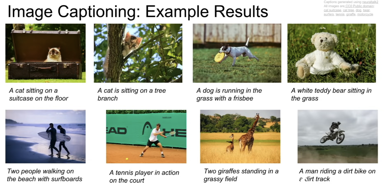
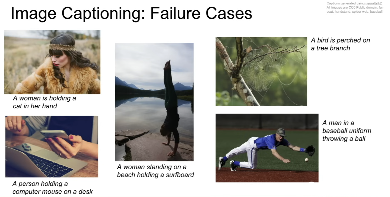
• if you try to run them on the data that was very different from the training data, they don't work well

Image Captioning with Attention

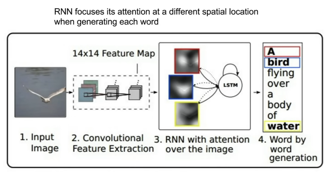
• now, when we're generating the words of this caption, we can allow the model to steer it's attention to different parts of the image

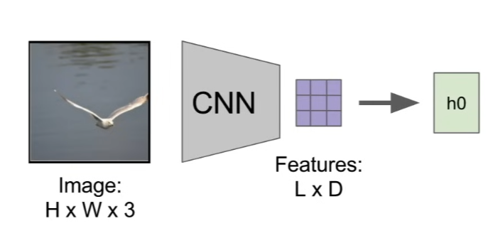
• our ConvNet, rather than producing a single vector and summarizing the entire image, it produces a grid of vectors that give maybe 1 vector for each spatial location in the image

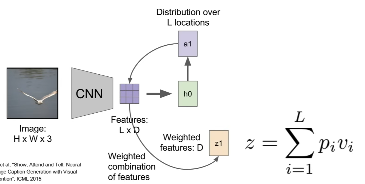
• when we run this model forward, in addition to sampling the vocabulary at every time step, it also produces a distribution over the locations in the image where it wants to look
  • this distribution over image locations can be seen as a kind of a tension of where the model should look during training
• now that 1st hidden state computes the distribution over image locations, goes back to the set of vectors to give a single summary vector that maybe focuses the attention on one part of that image

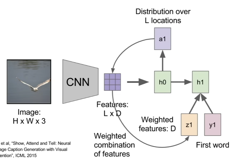
• now that summary vector gets fed as an additional input at the next time step
  
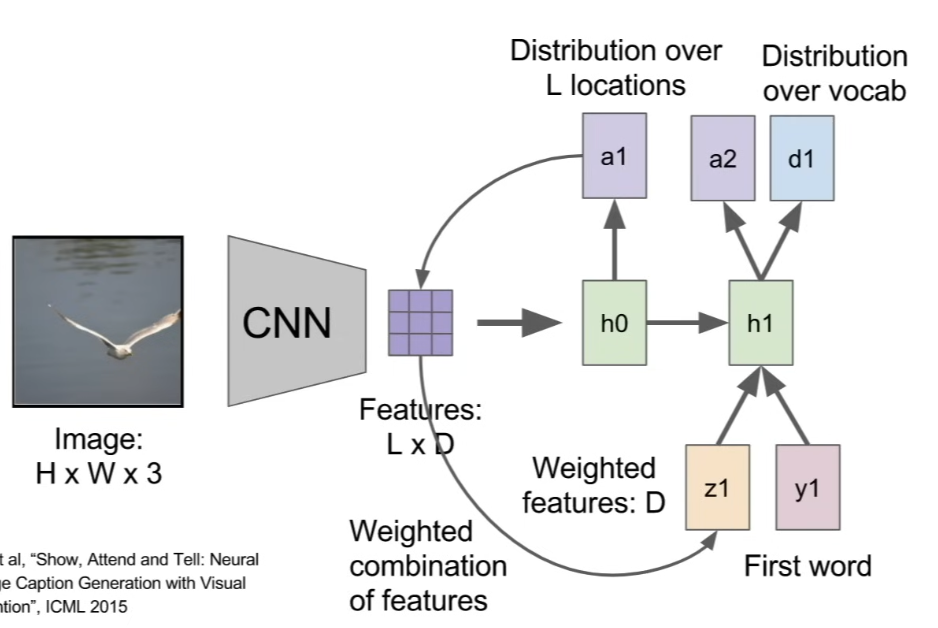
• and it will produce 2 outputs; a distribution over vocabulary words and a distribution over image locations
  
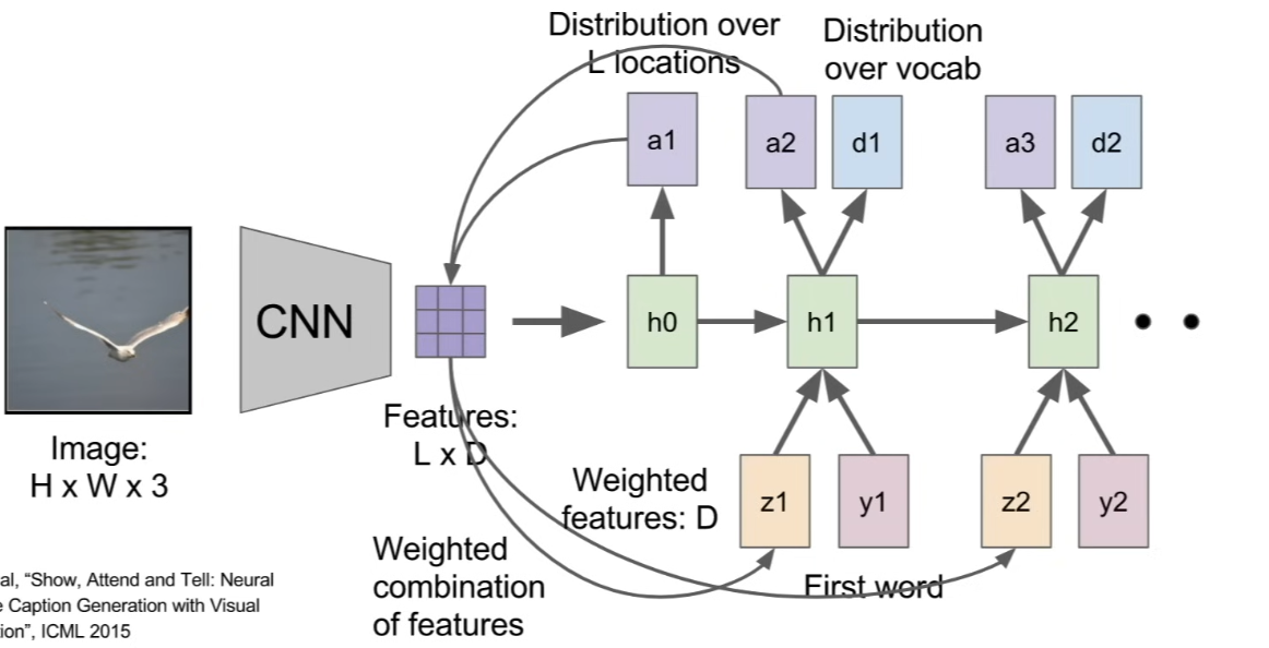
• the whole process will continue, and it will do 2 different things at every time step

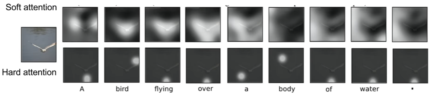
• after training, you can see that it shifts it's attention around the image for every word that it generates in the caption
• hard attention vs. soft attention
  • hard attention: forcing the model to select only 1 location to look at in the image at each time step
    • more tricky, because it's not a differentiable function
  • soft attention: taking a weighted combination of all features from all image locations

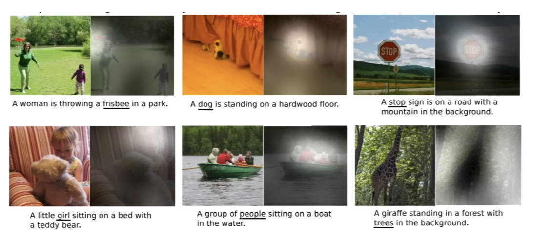
• tends to focus its attention on salient(가장 중요한, 핵심적인) or semantically(의미상으로) meaningful part of the image
  • when the model generated the word 'frisbee', at the same time, it was focusing its attention on the image region that contains frisbee
• b/c everything in this model is differentiable, b/c we can backprop through all of soft attention steps, all of the soft attention stuff comes out through the training process

Visual Question Answering

• idea of RNN and attention gets used in other tasks beyond image captioning
  
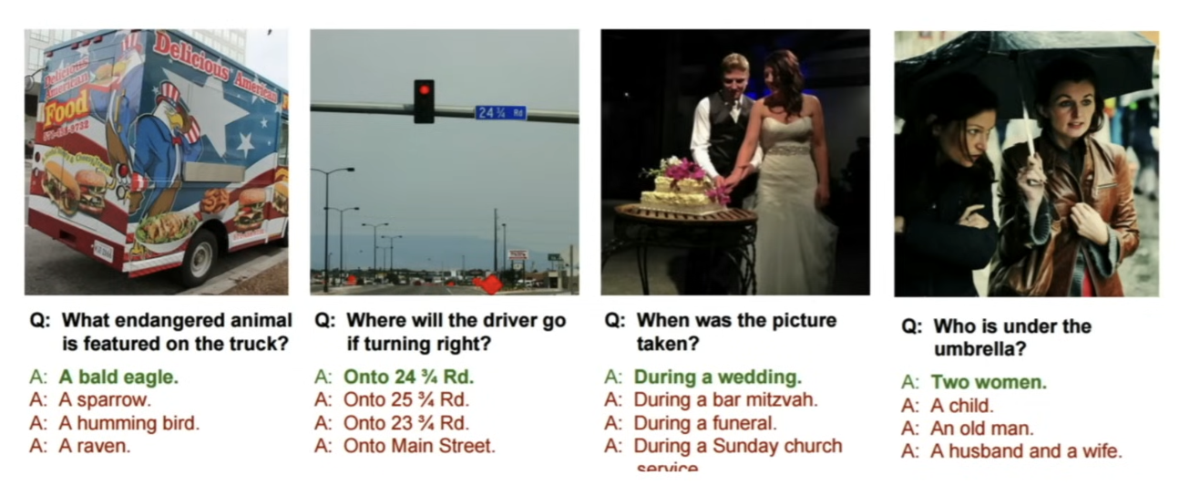
• here, the model takes 2 things as input; an image and a natural language question that's asking some question about the image

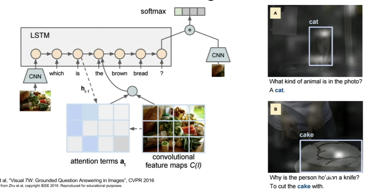
• stitching this model together using CNNs and RNNs
• many-to-one scenario
  • take the natural language sequence as an input → running RNN over each element of that input question, to summarize the input question in a single vector
  • have a CNN → to summarize the image
  • combine both the vectors from the CNN and RNN to predict a distribution over answers

Multilayer RNNs

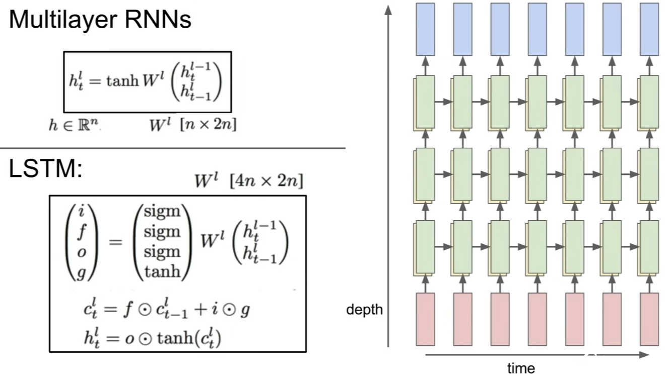
• 3-layer RNN
  • input goes in and produces a sequence of hidden states from the 1st RNN layer
  • then we have a sequence of hidden states
  • now we can use the sequence of hidden states as the input sequence for another RNN layer, which then produces another hidden state sequence
• stack these things on top of each other, since we know that in other contexts, deeper models tend to perform better for various problems (same holds in RNNs as well)
• 2, 3, 4 layer RNN is common
  • super deep models in RNNs are not common

Vanilla RNN Gradient Flow

• now that we know what kind of problems these RNNs can be used for, think about exactly what happens to these models when we try to train them

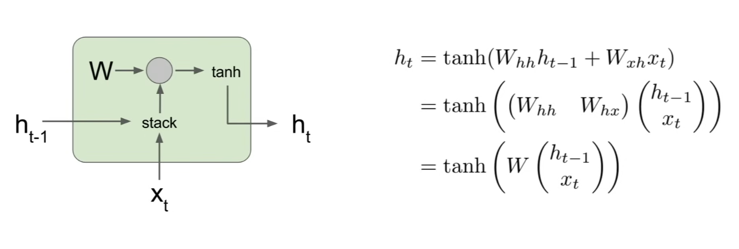
• here, take the current input $x_t$ and previous hidden state $h_{t-1}$ (these are vectors)
• stack them together
• perform matrix multiplication with $W$ matrix
• then squash that output through a $\tanh$, which gives us next hidden state

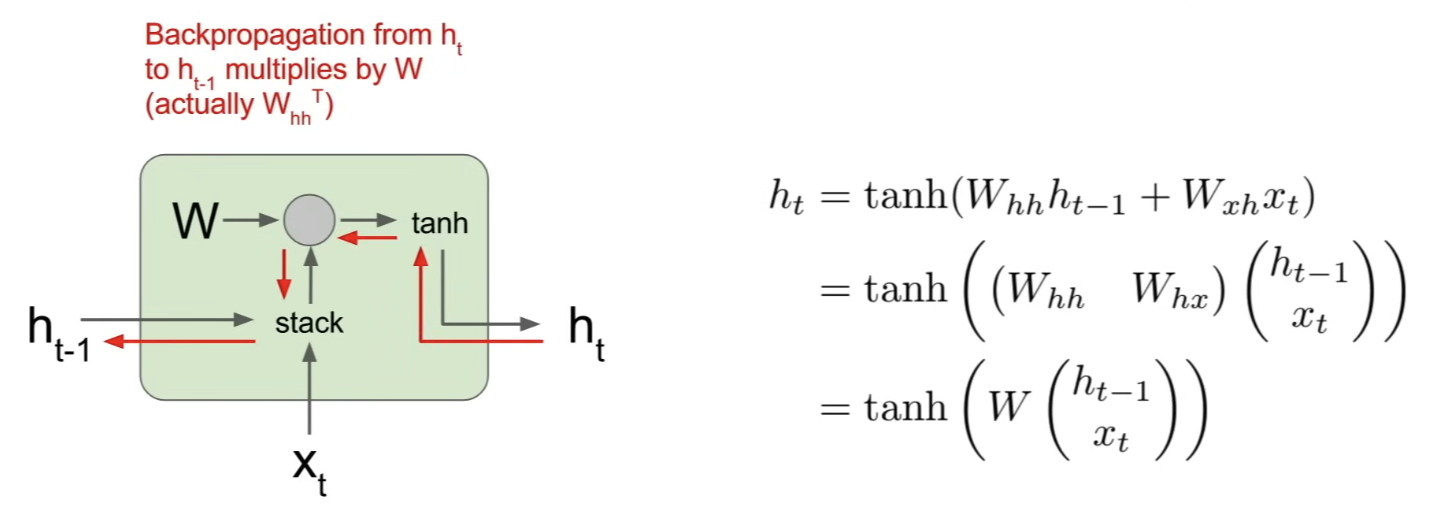
• during the backward pass, we'll receive the derivative of loss with respect to $h_t$
• and through the cell, we'll need to compute derivative of loss with respect to $h_{t-1}$
• gradient flows through the red path
  • when backpropping through matrix multiplication gate, you end up multiplying by the transpose of the Weight matrix
  • which means that everytime we backprop through RNN cells, we end up multiplying by some part of the weight matrix

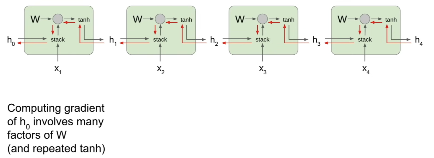
• What happens to the gradient flow through a sequence of these layers?
• now, when we want to compute the gradient of loss with respect to $h_0$, we need to backprop through every one of these RNN cells
  - and every time doing backprop, you'll pick up one of these $W^T$ factors
  - meaning that the final expression for gradient on $h_0$ will involve many factors of Weight matrix -> might be bad
  
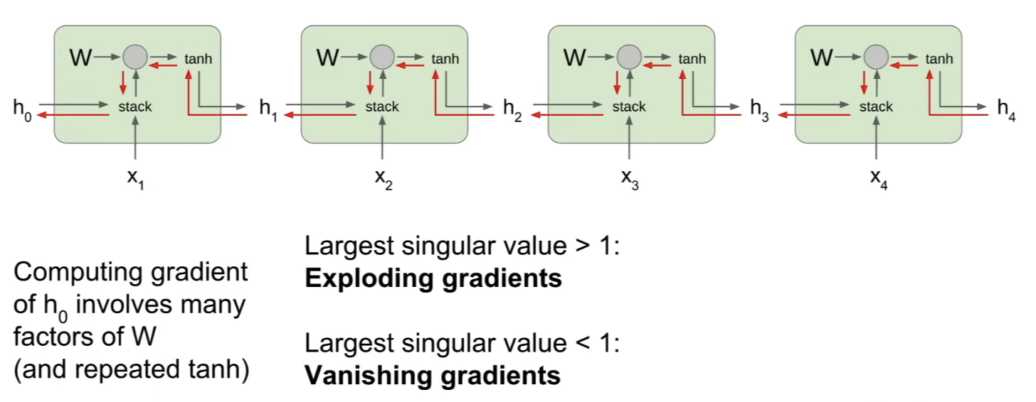
• But if we have a scalar and we multiply by that same number over and over again, multiplying by the same number over and over again is bad
  - in the scalar case, it's either going to explode if |number| > 1 or vanish toward 0 if |number| < 1
  • the only way in which this will not happen is if that number = 1, rare to happen in practice
• This same intuition extends to the matrix case, but now instead of the absolute value, look at the largest singular value of the $W$ matrix
  
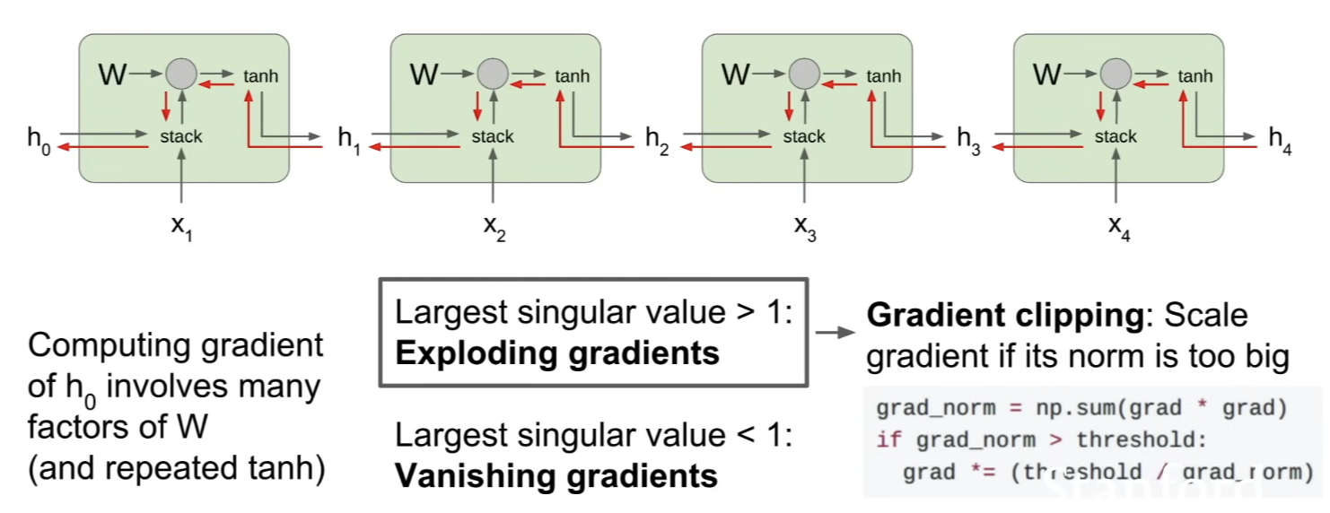
• Hack for Exploding Gradients problem
  - after computing gradient,
  - if gradient's L2 norm is above some threshold, clamp it down so it has the maximum threshold
  
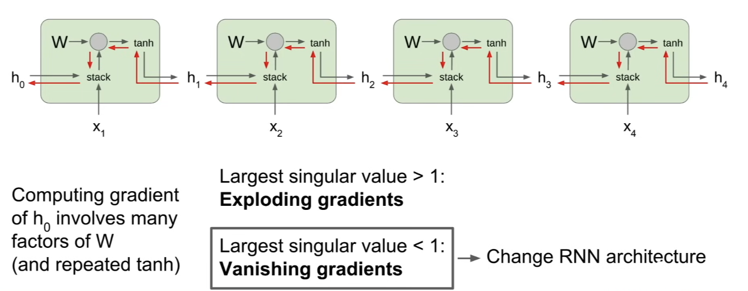
• For Vanishing Gradient problem,
  - we might need to move to a more complicated RNN architecture
  => motivates the idea of an LSTM

Long Short Term Memory (LSTM)

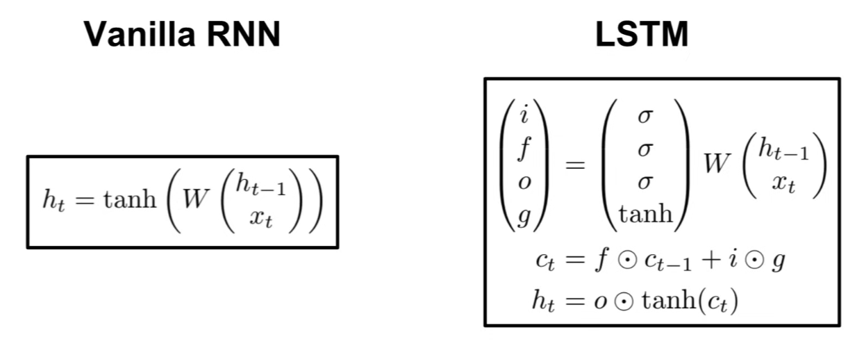
• slightly fancier recurrence relation for RNN
• designed to help alleviate the problem of vanishing and exploding gradients
• in Vanilla RNN,
  - it has hidden state
  • we used this recurrence relation to update the hidden state at every time step
• in LSTM,
  - maintain 2 hidden states at every time step; $h_t$ and $c_t$
  • $h_t$: hidden state
  • $c_t$: cell state; a vector kept inside the LSTM, and does not get exposed to outside world
• take 2 inputs, use them to compute 4 gates ($i$, $f$, $o$, $g$)
• use those gates to update cell state $c_t$, and expose part of the cell state as the hidden state at the next time step

Architecture

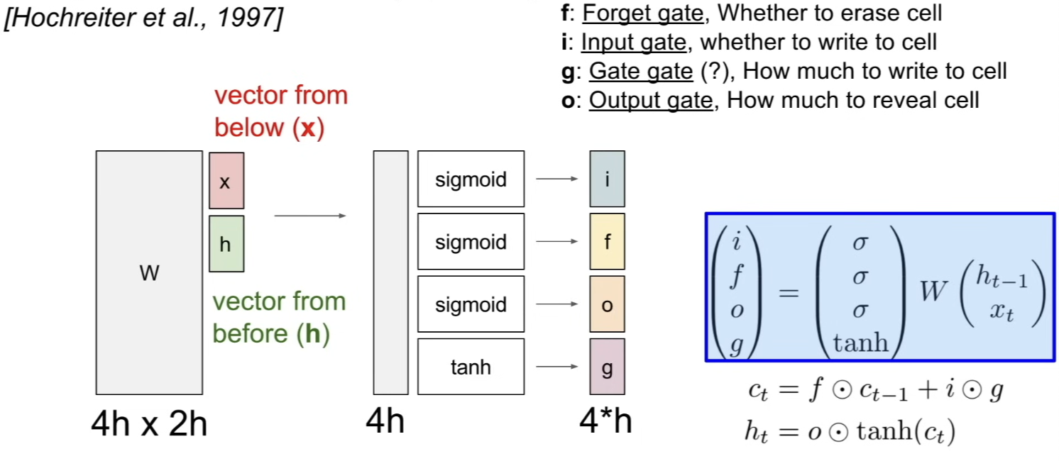
1. Given previous hidden state $h_t$ and current input vector $x_t$ (like vanilla RNN), stack them
2. multiply by a very big weight matrix $W$, to compute 4 different gates
- $i$: input gate, how much do we want to input into our cell
- $f$: Forget gate, how much do we want to forget the cell memory from the previous time step
- $o$: Output gate, how much do we want to reveal ourself to the outside world
- $g$: ?? gate, how much do we want to write into our input cell
- these gates use different non-linearity; $i$,$f$,$o$ use sigmoids, which means their values will be between 0 and 1; $g$ use $\tanh$, which means its output will be between -1 and 1
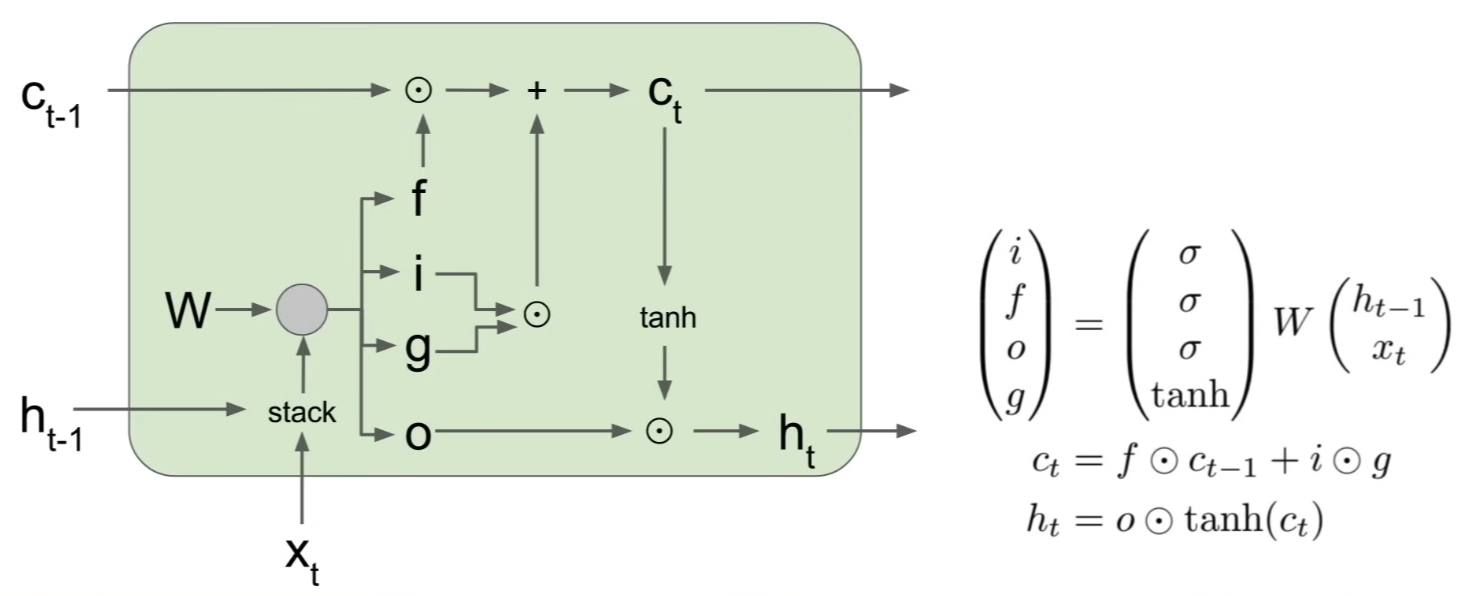
3. in the cell state equation, at every time step, the cell state has different independent scalar values, and they're all being incremented or decremented by 1
- so inside a cell state, we can either remember or forget the previous state, and either increment or decrement each element of that cell state by up to 1 at each time step
- elements of cell state can be interpreted as little scalar integer counters that can be incremented or decremented at each time step
4. Compute a hidden state
- use the updated cell state
- squash that counter value (elements of the cell state) into 0~1 range using a $\tanh$
- then, multiply element-wise by the output gate
- output gate is coming through a sigmoid, so it's mostly 0s and 1s
- output gate tells us for each element of our cell state, do we want to reveal or not reveal that element of the cell state when we're computing external hidden state

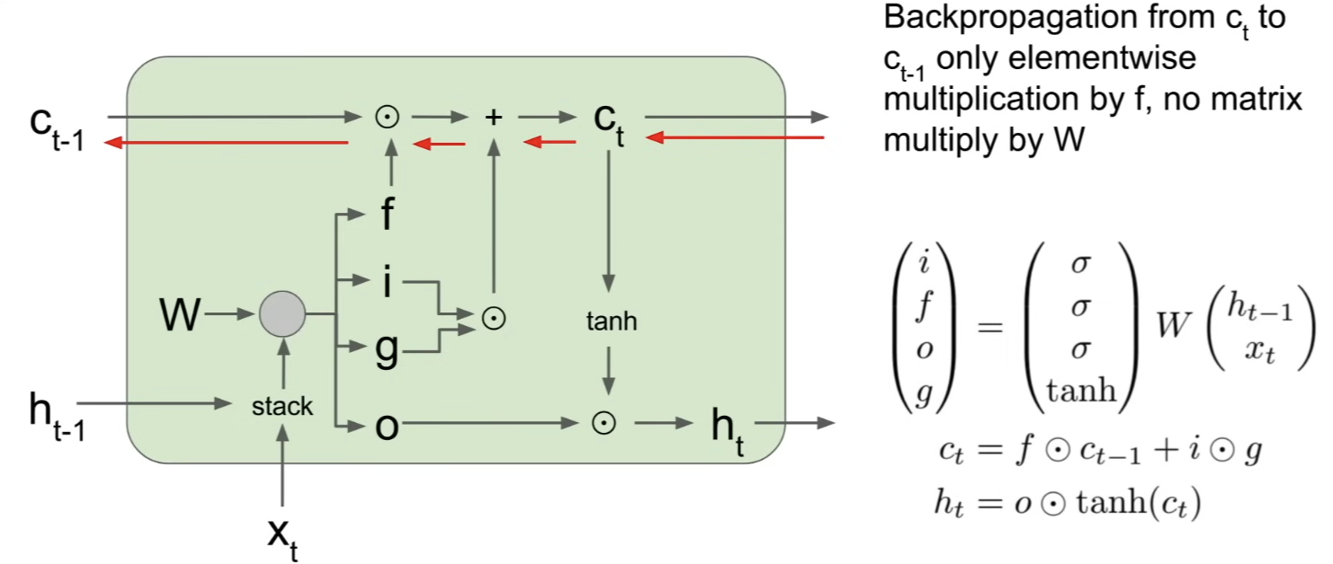
• in vanilla RNN, bad thing happen during backward pass, where we keep multiplying by the weight matrix $W$
• but in LSTM,
  - when we have upstream gradient and once we backprop backwards through addition operation, addition just copies that upstream gradient into 2 branches -> upstream gradient gets copied and directly passed back to the element wise multiply
  • upstream gradient ends up getting multiplied element wise by the forget gate
• as we backprop through this cell state, only thing that happens to upstream cell state gradient is that it ends up getting multiplied element-wisely by the forget gate
  => much lot nicer than vanilla RNN; forget gate is an element wise multiplcation rather than a full matrix multiplication and element wise multiplication will potentially be multiplying by a different forget gate at every time step, but the forget gate can vary at each time step(avoiding exploding/vanishing gradient)

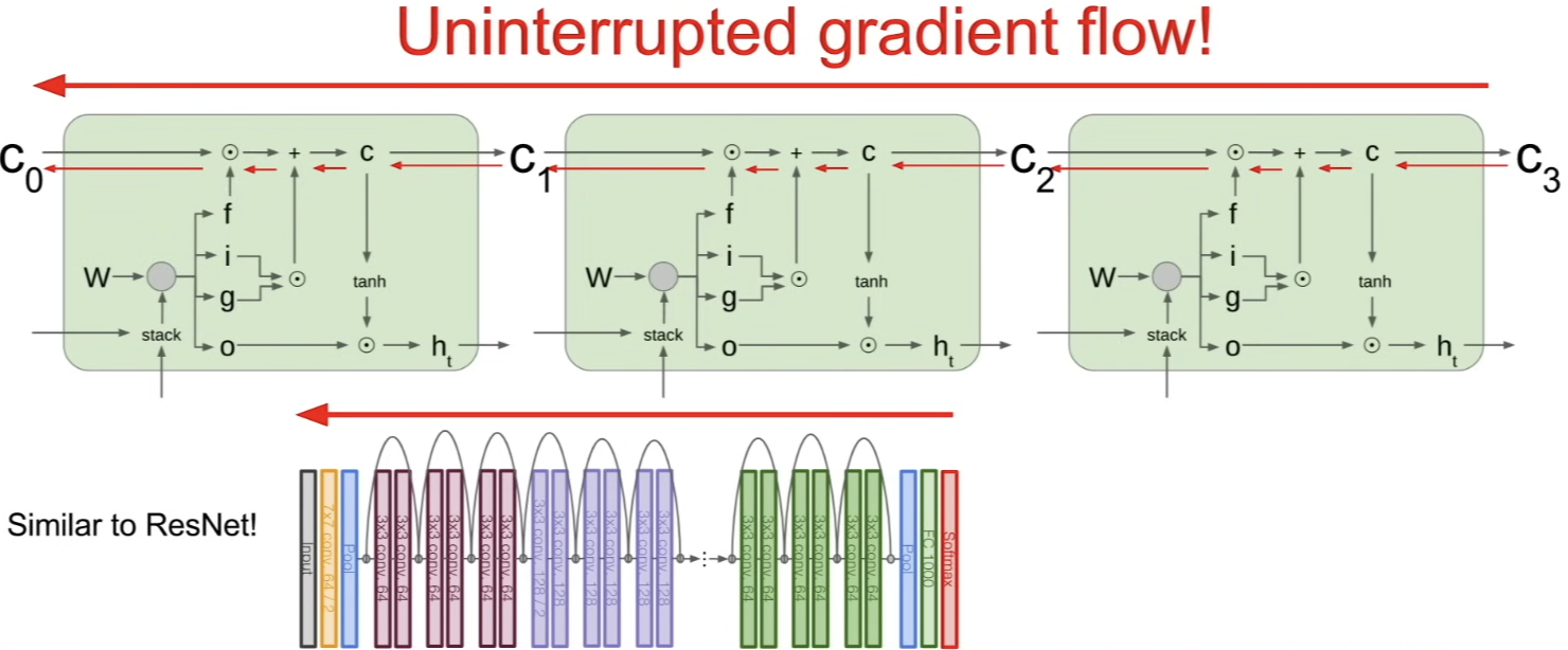
• highway networks; at every layer, compute a candidate activation as well as a gate function that interpolates between our previous input at that layer and that candidate activation that came through Conv or whatnot

Summary

• RNNs allow a lot of flxibility in architecture design
• Vanilla RNNs are simple but don't work very well
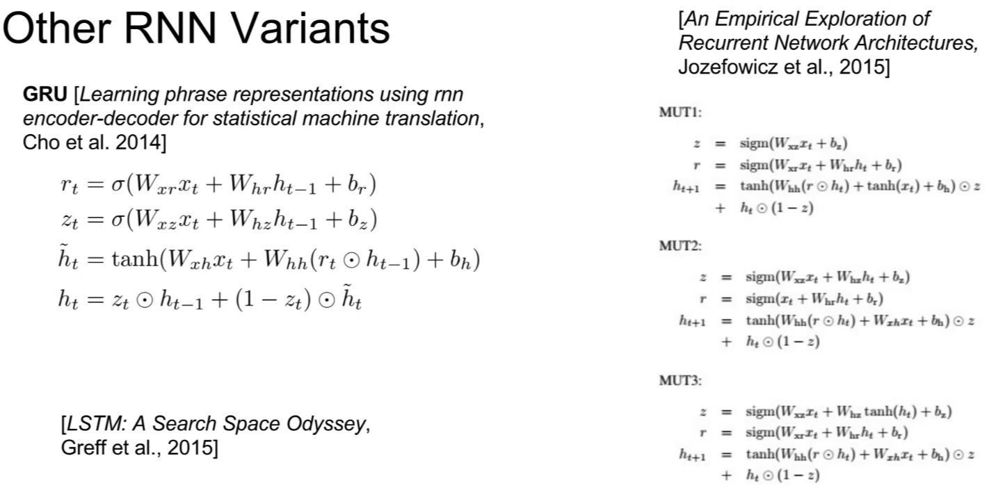
• Common to use LSTM or GRU: their additive interactions improve gradient flow
• Backward flow of gradients in RNN can explode or vanish. Exploding is controlled with gradient clipping. Vanishing is controlled with additive interactions (LSTM)
• Better/Simpler architectures are a hot topic of current research
• Better understanding (both theoretical and empirical) is needed.