🔎 Stanford CS231n 강의를 듣고 기록용도로 정리하는 게시글입니다.

Reinforcement Learning

• Problems involving an agent interacting with an environment, which provides numeric reward signals
• Goal: Learn how to take actions in order to maximize reward

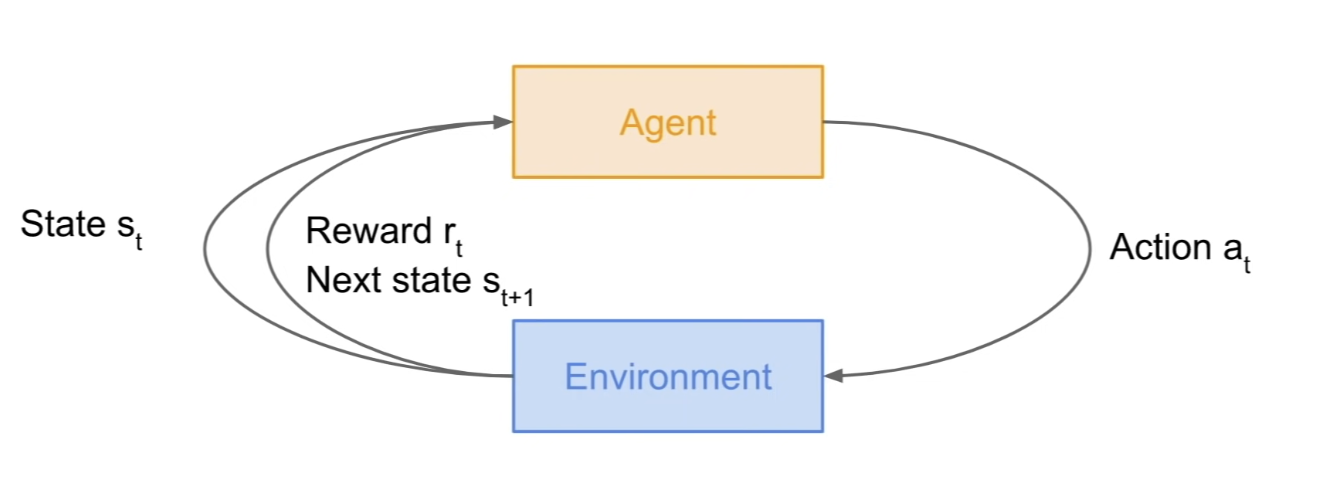
• environment gives the agent a state
• agent takes an action
• environment gives back a reward and the next state
• keep going on in this loop on and on, until the environment gives back a terminal state, which ends the episode

Classic RL Problems

Cart-Pole Problem

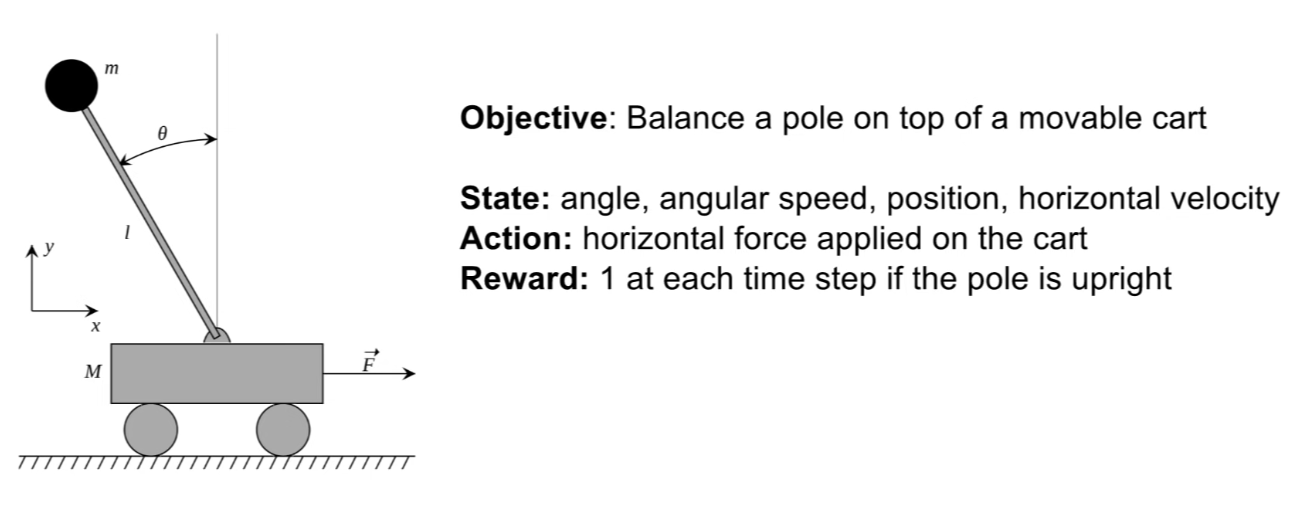
• state = description of the system

Robot Locomotion

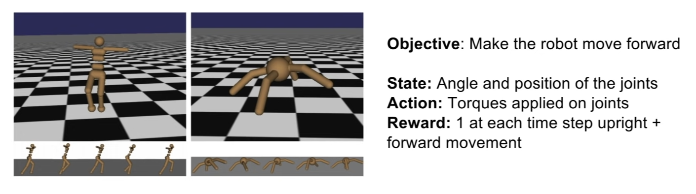
• torque: 회전력

Atari Games

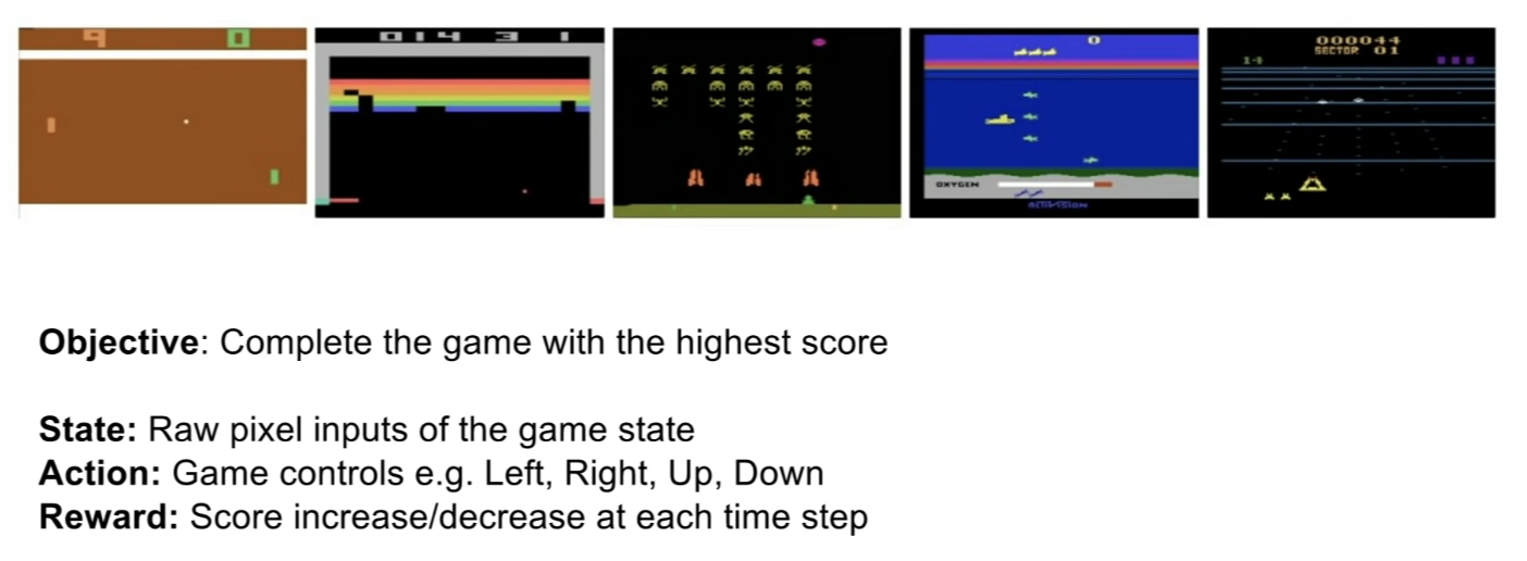
• agent = a player that's playing these games

Go

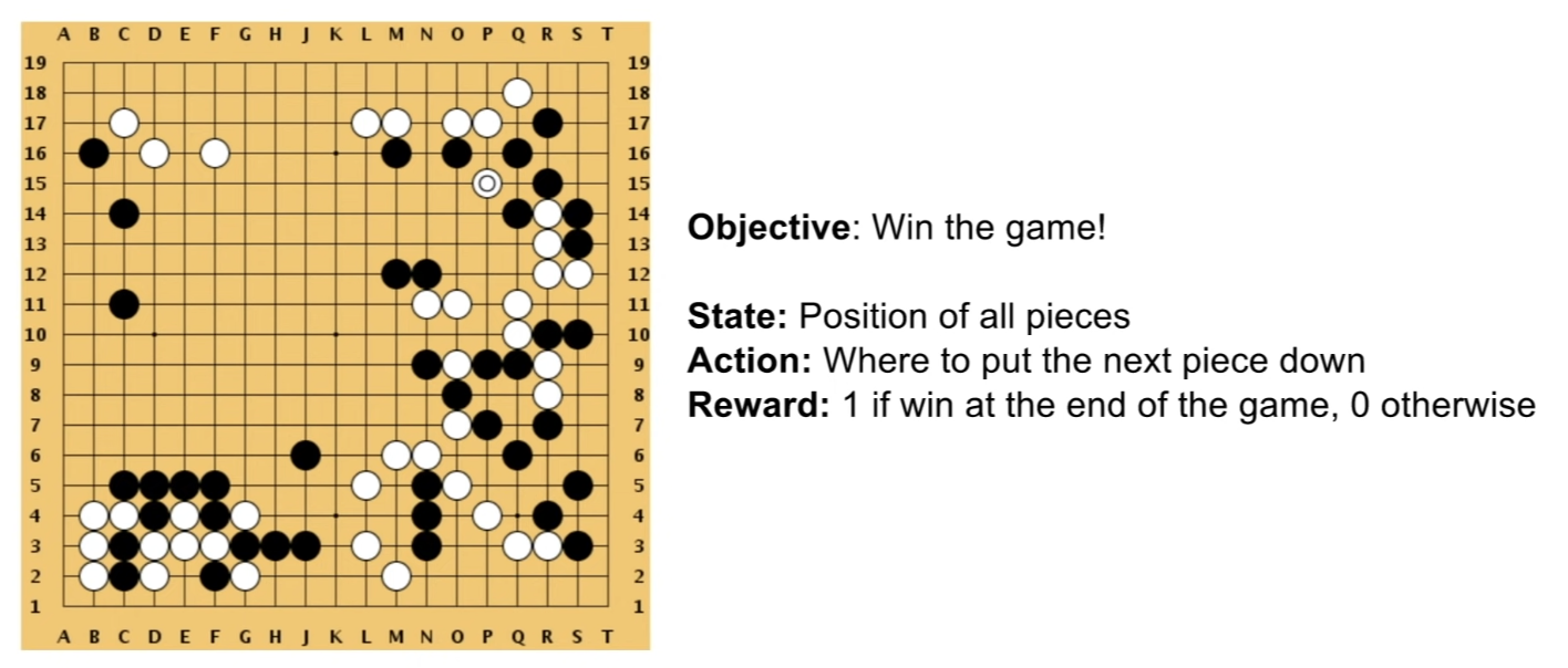
Markov Decision Process

• Mathematical formulation of the RL problem
• Markov property: Current state completely charaterises the state of the world
• MDP is defined by: $(\mathcal{S}, \mathcal{A}, \mathcal{R}, \mathbb{P}, \gamma)$
  - $\mathcal{S}$: set of possible states
  • $\mathcal{A}$: set of possible actions
  • $\mathcal{R}$: distribution of reward given (state, action) pair
    • function mapping from state, action to reward
  • $\mathbb{P}$: transition probability i.e.(즉) distribution over next state given (state, action) pair
  • $\gamma$: discount factor
    • how much we value rewards coming up soon versus later on

How this works

• At time step t = 0 (initial time step), environment samples initial states $s_0 ~ p(s_0)$
  - sample $s_0$ from the initial state distribution $p(s_0)$
• Then, from t = 0 until done:
  - Agent selects action $a_t$
  • Environment samples reward $r_t ~ R(.|s_t,a_t)$
    • reward given the state and action you just took)
  • Environment samples next state $s_{t+1} ~ P(.|s_t, a_t)$
    • given the probability distribution
  • Agent receives reward $r_t$ and next state $s_{t+1}$
• A policy $\pi$ is a function from $\mathcal{S}$ to $\mathcal{A}$ that specifies what action to take in each state
  - this can be either deterministic or stochastic
• Objective: find policy $\pi^*$ that maximizes cumulative discounted reward: $\displaystyle\sum_{t>0}\gamma^tr_t$
  - $\pi^*$ is the optimal policy

A simple MDP: Grid World

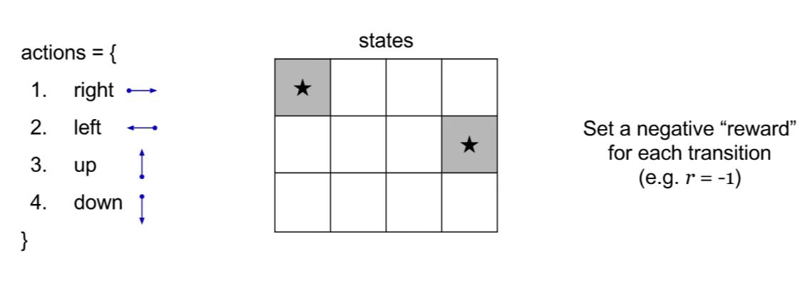
• objective: reach one of terminal state (greyed out) in least number of actions

• random policy and optimal policy
  
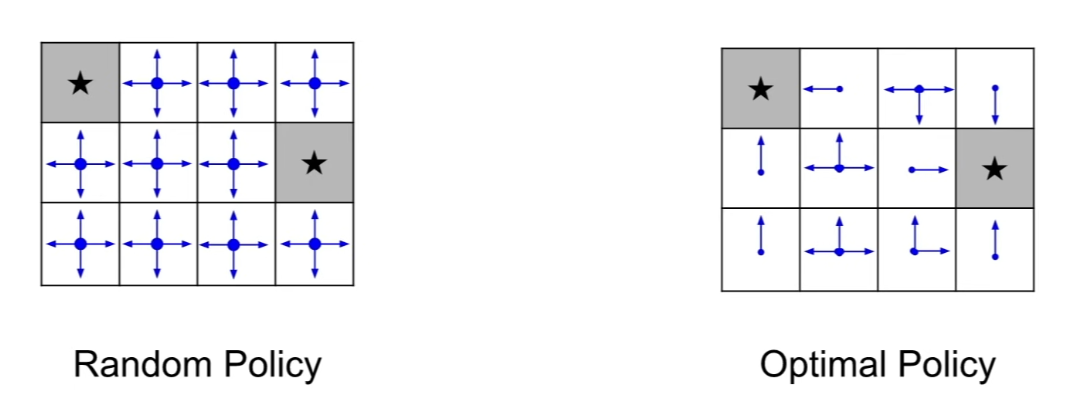
  - random policy: at any given state or cell that you're in, samples randomly which direction you'll move in next (all of those have equal probability)

  • optimal policy: take the action, the direction that moves us closest to the a terminal state

Optimal Policy

• We want to find optimal policy $\pi^*$ that maximizes the sum of rewards
  - optimal policy will tell us given any state, what the action we should take in order to maximize the sum of the rewards that we'll get is
• How do we handle the randomness in MDP? (initial state, transition probability...)
  - => maximize the expected sum of the rewards
  • Formally: $\displaystyle\pi^* = \arg \max_\pi\mathbb{E}\Biggr[\sum_{t\ge0}\gamma^tr_t|\pi\Biggr]$ with $s_0~p(s_0), a_t~\pi(\cdot|s_t), s_{t+1} ~ p(\cdot|s_t,a_t)$
    - maximizing this expected sum of future rewards over $\pi$, where we have initial state sampled from our state distribution, actions sampled from policy given the state, and the next state sampled from transition probability distributions.

Definitions

• As we follow the policy, we'll sample trajectories(paths) for every episodes $s_0,a_0,r_0, s_1, a_1, r_1, ...$
• Value function: at state $s$, the expected cumulative reward from following the policy from state $s$
  - "How good is a state?"
  • $\displaystyle V^\pi(s) = \mathbb{E}\Biggr[\sum_{t\ge0}\gamma^tr_t|s_0=s,\pi\Biggr]$
• Q-value function: at state $s$, and action $a$, the expected cumulative reward from taking action $a$ in state $s$ and then following the policy
  - "How good is a state-action pair?"
  • $\displaystyle Q^\pi(s,a) = \mathbb{E}\Biggr[\sum_{t\ge0}\gamma^tr_t|s_0=s,a_0=a,\pi\Biggr]$
• the optimal Q-value function $Q^*$ is the maximum expected cumulative reward achievable from a given (state, action) pair
  • $\displaystyle Q^*(s,a) = \max_\pi \mathbb{E}\Biggr[\sum_{t\ge0}\gamma^tr_t|s_0=s,a_0=a,\pi\Biggr]$
• $Q^*$ satisfies the Bellman equation
  • $\displaystyle Q^*(s,a) = \mathbb{E}_{s'\sim \epsilon} \Biggr[r+\gamma\max_{a'}Q^*(s', a')|s,a \Biggr]$
  • given any (state, action) pair $s$ and $a$, the value of this pair will be the reward that you'll get, $r$, plus the value of whatever state you end up in($s'$)
  • since we know that we have the optimal policy, we also know that we'll play the best action that we can at state $s'$
    • then, the value at $s'$ will be the maximum over the actions, $a'$, of $Q^*$ at $s'$,$a'$
  • as always, we have expectation, b/c we have randomness over what state we'll end up in
• Intuition: if the optimal state-action values for the next time-step $Q^*(s',a')$ are known, then the optimal strategy is to take the action that maximizes the expected value of $r+\gamma Q^*(s',a')$
  - $Q^*$ will tell us the maximum future reward that we can get from any of the actions, so we should take a policy that's following this and take the action that's going to lead to best forward
  • so, the optimal policy $\pi^*$ corresponds to taking the best action in any state as specified by $Q^*$

Solving for the optimal policy

• Value iteration algorithm: Use Bellman equation as an iterative update
  - $\displaystyle Q_{i+1}(s,a) = \mathbb{E}\Biggr[r+\gamma\max_{a'}Q_i(s',a')|s,a\Biggr]$
  • at each step, refine approximation of $Q^*$ by trying to enforce the Bellman Equation
  • under some mathematical conditions, we know that $Q_i$ will converge to $Q^*$ as i approchaes infinity
    - What's the problem with this?
    • Not scalable. We have to compute Q(s,a) for every (state, action) pair in order to make iterative updates. If state is current game state pixels, computationally infeasible(실행불가능) to compute for entire state space!
  • Solution: use a function approximator to estimate $Q(s,a)$, for example, a neural network
    • anytime if we have some really complex function we don't we want to estimate, a neural networks is a good way to estimate this
      - => Q-learning

Q-Learning (Solving optimal policy)

• Use a function approximator to estimate the action-value function
  - $Q(s,a;\theta) \approx Q^*(s,a)$
  - $\theta$ is the function parameters (weights)
• If the function approximator is a deep neural network => deep q-learning
  - been used recently
• Remember: we want to find a Q-fuction that satisfies the Bellman Equation
  - $\displaystyle Q^*(s,a) = \mathbb{E}_{s'\sim \epsilon} \Biggr[r+\gamma\max_{a'}Q^*(s', a')|s,a \Biggr]$
  • we want the Bellman Equation to happen
• Forward pass
  - We can train this where the loss function is going to try and minimize the error of the Bellman Equation (= how far $Q(s,a)$ is from its target, which is $Y_i$ here
  • Take the forward passes of the loss function, trying to minimize error,
  • Loss function: $L_i(\theta_i) = \mathbb{E}_{s,a\sim\rho(\cdot)} \bigr[(y_i-Q(s,a;\theta_i))^2\bigr]$ where $y_i = \mathbb{E}_{s'\sim\epsilon}\biggr[r+\gamma\max_{a'}Q(s',a';\theta_{i-1})|s,a\biggr]$
• Backward pass
  - Take the gradient of the loss, with respect to our network parameter, $\theta$
  • Gradient update (with respect to Q-function parameters $\theta$)
  • $\nabla{\theta_i}L_i(\theta_i) = \mathbb{E}_{s,a\sim\rho(\cdot);s'\sim\epsilon}\Biggr[r+\gamma\max_{a'}Q(s',a';\theta_{i-1})-Q(s,a;\theta_i))\nabla_{\theta_i}Q(s,a;\theta_i)\Biggr]$
• Goal: to have this effect as we're taking gradient steps of iteratively trying to make Q-function closer to the target value($y_i)

Q-network Architecture

• $Q(s,a;\theta)$: neural network with weights $\theta$
  
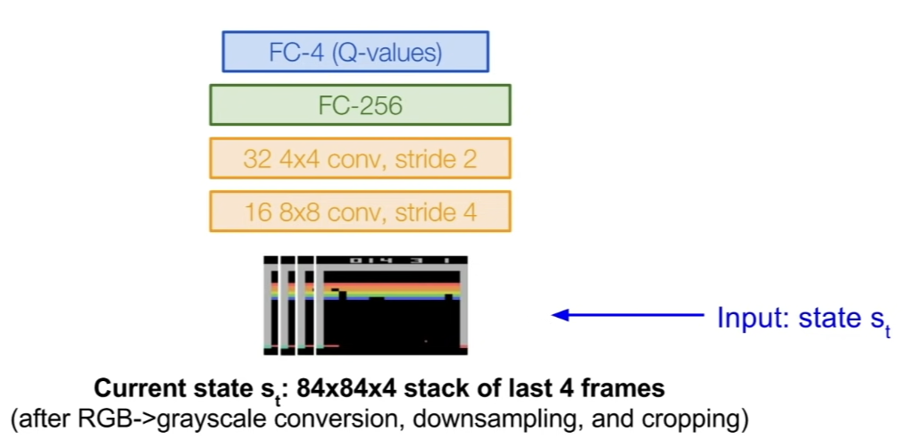
  - input: state $s-t$ is current game screen
  - in practice, we'll take a stack of the last 4 frames, so we have some history
  - take raw pixel values, and do some preprocessings(RGB to gray-scale conversions, downsampling, and cropping)
  - we'll get 84x84x4 staks of the last 4 frames by this
  - on top of this, we have conv layers, fully connected layers...
  - Last FC layer has 4-d output (if 4 actions)
  - corresponding to $Q(s_t,a_1), Q(s_t,a_2), Q(s_t,a_3), Q(s_t,a_4)$ (Q-value for each action, given the input state)
  - this is 1 scalar value for each of the actions
• Using this network structure, a single feedforward pass can compute Q-values for all actions from the current state => efficient
  - taking the current state in, b/c we have the Q-value for each action as an output layer, we can just do 1 pass and get all of these values out
• To train this, we'll use the loss function from before

Training Q-network: Experience Replay

• Learning from batches of consecutive(연이은) samples is problematic:
  - Samples are correlated
  => inefficient learning
  • Current Q-network parameters determines next training samples (e.g. if maximizing action is to move left, training samples will be dominated by samples from left-hand side)
    => can lead to bad feedback loops
• Address these problems by using experience replay
  - Continually update a replay memory table of transitions($s_t, a_t, r_t, s_{t+1}$) as game(=experience) episodes are played
  • Train Q-network on random minibatches of transitions from the replay memory, instead of consecutive samples
  • Each transition can also contribute to mutiple weight updates
    => greater data efficiency

Deep Q-Learning with Expereicne Replay

• Putting it together
  
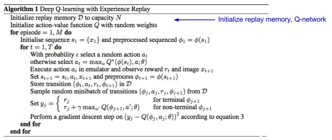
  - initialize replay memory to some capacity N (that we choose) and initialize Q-network with random weights
  
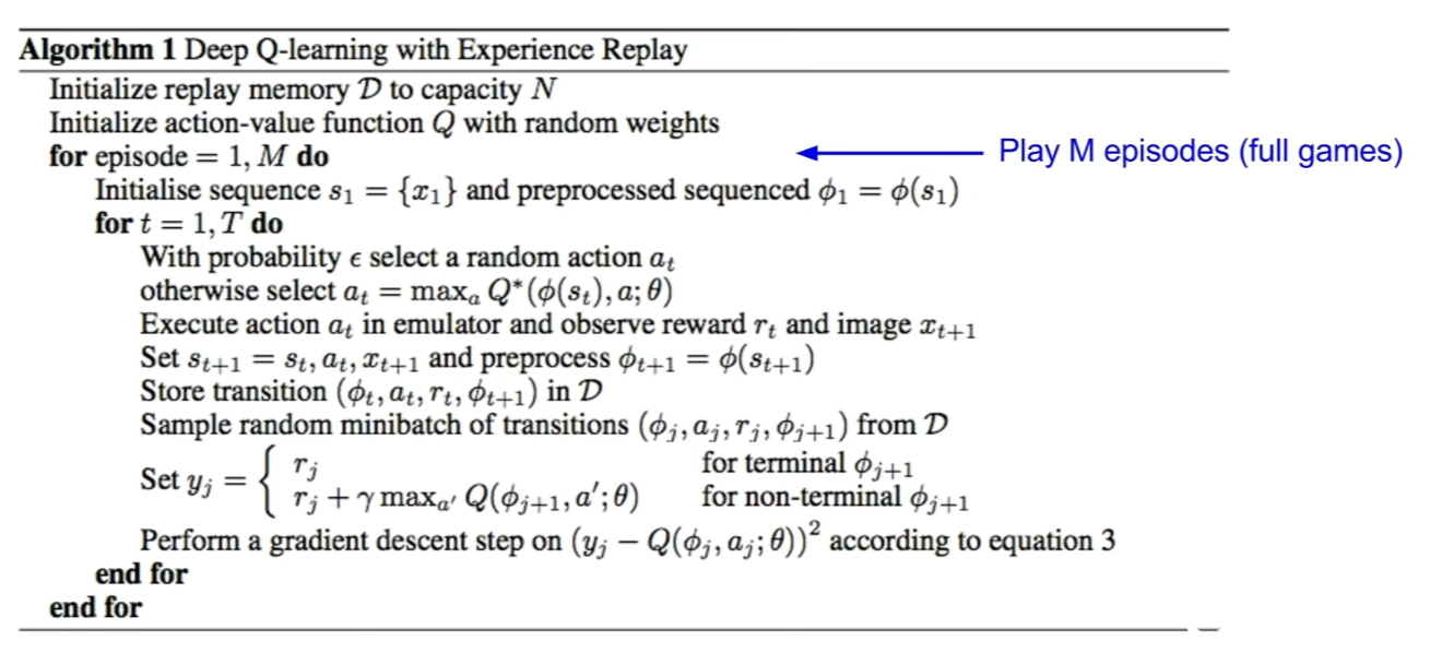
  - training episodes
  
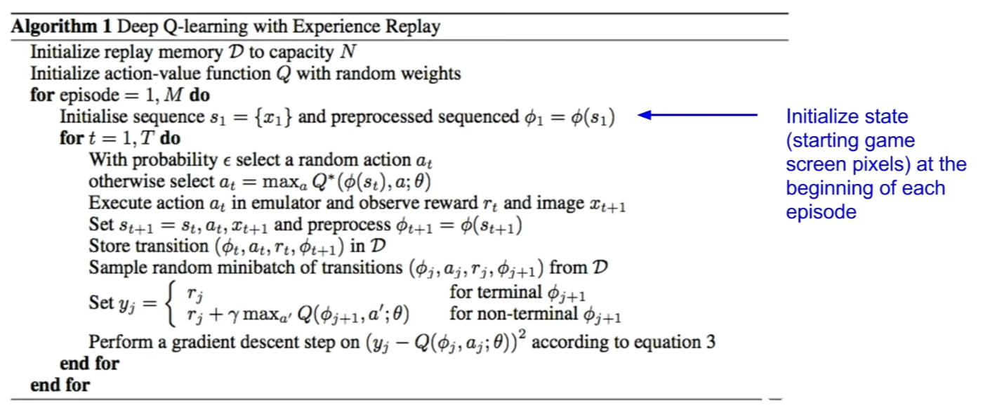
• initialize state (=starting game screen pixels)
• have to go through preprocessing step to get to an actual input state
  
  
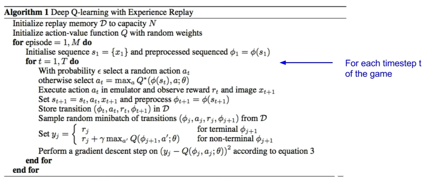
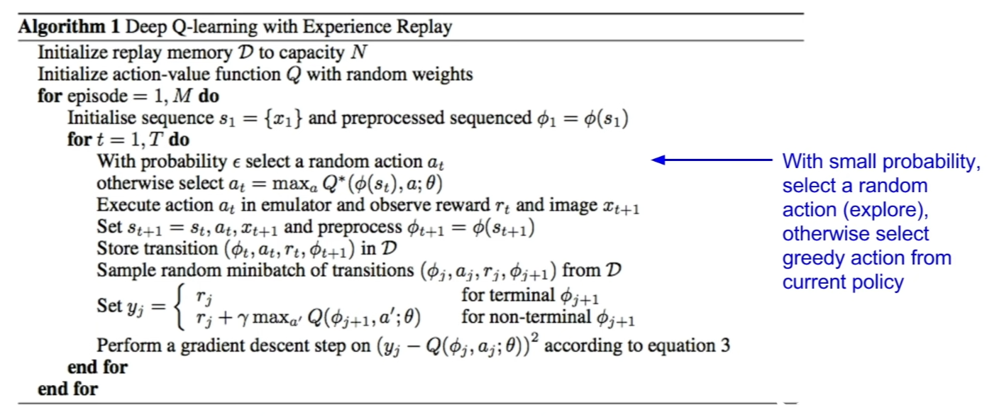
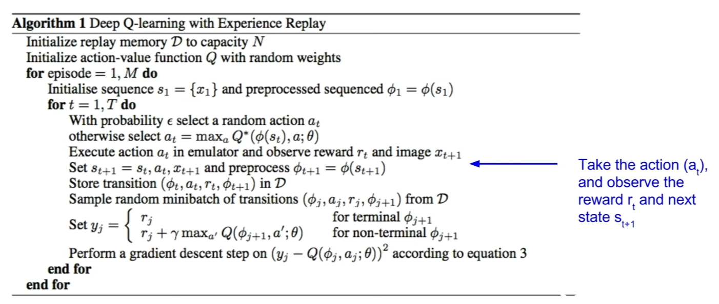
• one thing important here is to have sufficient exploration, so we want to make sure that we're sampling different parts of the state space
• so, for each time step,
  - with small probability, select a random action
  - otherwise, select greedy action from current policy (most of the time...)
  
  
  
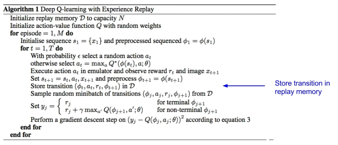
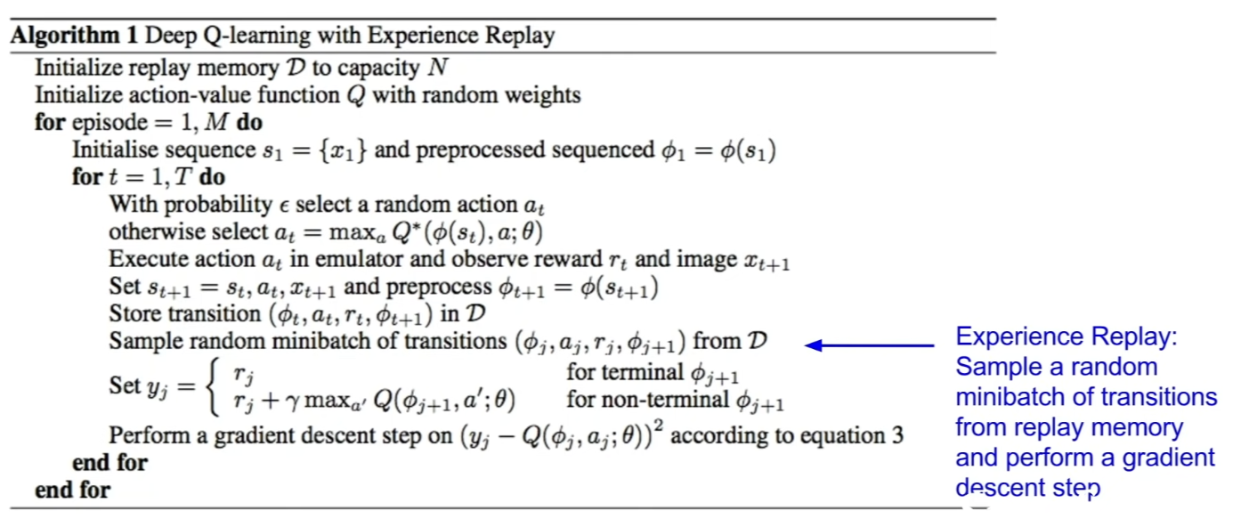
• train a network little bit; do experience replay
  - take a sample of random mini-batch of transitions that we have from the replay memory
  • perform a gradient descent step upon this

Policy Gradients

• Problem with Q-Learning?
  - Q-function can be very complicated
  • ex) a robot grasping an object has a very high-dimensional state => hard to learn exact value of every (state, action) pair
  • But, policy can be much simpler: just close your hand
  • Can we learn a policy directly, e.g. finding the best policy from a collection of policies?
    => Policy Gradients
• Formally, let's define a class of parametrized policies: $\Pi = \{\pi_\theta, \theta \in \mathbb{R}^m\}$
  - parametrized by weights $\theta$
• For each policy, define its value:
  - $\displaystyle J(\theta)=\mathbb{E}\Biggr[\sum_{t\ge0}\gamma^tr_t|\pi_\theta\Biggr]$
  • J is expected cumulative sum of future rewards that we care about
• Goal: find the optimal policy $\displaystyle\theta^*=\arg\max_\theta J(\theta)$
  - How? -> Gradient ascent on policy paramers!

REINFORCE algorithm

• Mathematically, we can write the expected future reward over trajectories
  $\begin{aligned} J(\theta) & = \mathbb{E}_{\tau\sim p(\tau;\theta)} \big[r(\tau)\big] \\ & = \int_\tau r(\tau)p(\tau;\theta)d\tau \end{aligned}$
  - sample trajectories of experiece, e.g. episodes of game play
  • where $r(\tau)$ is the reward of a trajectory $\tau = (s_0, a_0, r_0, s_1, ...)$
  • so, for each trajectory, we can compute a reward for that trajectory (=cumulative reward that we got from following this trajectory)
  • value of the policy, $\Pi_\theta$ is the expected reward of these trajectories we can get from following $\Pi_\theta$
• We want to do a gradient ascent -> so, differentiate this
  - $\nabla_\theta J(\theta) = \int_\tau r(\tau) \nabla_\theta p(\tau;\theta)d\tau$
  • But, this is intractable. Gradient of an expectation is problematic when p depends on $\theta$
    • b/c here, we want to take the gradient of $p(\tau;\theta)$ (p of $\tau$, given $\theta$)
      • but we want to take this integral over $\tau$
• However, we can use a nice trick
  - $\displaystyle\nabla_\theta p(\tau;\theta) = p(\tau;\theta) \frac{\nabla_\theta p(\tau;\theta)}{p(\tau;\theta)} = p(\tau;\theta)\nabla_\theta \log p(\tau;\theta)$
  • trick: taking the gradient that we want, of $p$ -> rewrite this by multiplying by $\displaystyle 1 = \frac{p(\tau;\theta)}{p(\tau;\theta)}$
    • b/c gradient of the $\log p$ is $\displaystyle \frac{1}{p \times \nabla_p}$
  • if we inject this back:
    • $\displaystyle \begin{aligned} \nabla_\theta J(\theta) & = \int_\tau (r(\tau)\nabla_\theta \log p(\tau;\theta))p(\tau;\theta)d\tau \\ & = \mathbb{E}_{\tau \sim p(\tau;\theta)} \big[r(\tau)\nabla_\theta \log p(\tau;\theta)\big] \end{aligned}$
      - b/c now we have gradient of $\log p$ times the probabilities of all of the trajectories and then taking this integral over $\tau$,
      • this is now going to be an expectation over trajectories $\tau$
  • what we've done here; took a gradient of an expectation, and transformed it into an expectation of gradients
  • so, now we can use sampled trajectories that we can get, in order to estimate our gradient
    • do this by Monte Carlo sampling
• Can we compute those quantities without knowing the transition probabilities?
• We have: $\displaystyle p(\tau;\theta) = \prod_{t \ge 0} p(s_{t+1}|s_t,a_t)\pi_\theta(a_t|s_t)$
  - $p(\tau;\theta)$ = probability of a trajectory
  • is the product of all of the transition probabilities of the next state we get, given the current state and action
  • as well as probability of the action we took under policy $\pi$
• Thus: $\displaystyle \log p(\tau;\theta) = \sum_{t \ge 0} \log p(s_{t+1}|s_t, a_t) + \log \pi_\theta(a_t|s_t)$
  - 바로 위의 식에서 $\prod$안의 식에 $\log$를 취한 값임 (곱하기 -> 더하기)
• When differentiating: $\displaystyle \nabla_\theta \log p(\tau;\theta) = \sum_{t\ge0} \nabla_\theta \log \pi_\theta (a_t|s_t)$
  • we want to differentiate it with respect to $\theta$
    • but the first term has no $\theta$
  • only place where we have $\theta$ is the 2nd term
    => Doesn't depend on transition probabilities!
• Therefore, when sampling a trajectory $\tau$, we can estimate $J(\theta)$ with
  $\displaystyle \nabla_\theta J(\theta) \approx \sum_{t\ge0}r(\tau)\nabla_\theta \log \pi_\theta (a_t|s_t)$

Intution

• Gradient estimator: $\displaystyle \nabla_\theta J(\theta) \approx \sum_{t\ge0}r(\tau)\nabla_\theta \log \pi_\theta (a_t|s_t)$
• Interpretation:
  - If $r(\tau)$ is high, push up the probabilities of the actions seen
  • If $r(\tau)$ is low, push down the probabilities of the actions seen
• Might seem simplistic to say that if a trajectory is good then all its actions were good. But in expectation, it averages out!
  - so we have an unbiased estimator
• However, this also suffers from high variance because credit assignment is really hard. Can we help the estimator?
  - we're saying that given reward that we got, we'll say that all of the actions were good, and we'll hope that this assignment of which actions were actually the best actions, that mattered, are going to average out over time
  • we need to have a lot of samples to get a good estimate

Variance reduction

• Gradient estimator: $\displaystyle \nabla_\theta J(\theta) \approx \sum_{t\ge0}r(\tau)\nabla_\theta \log \pi_\theta (a_t|s_t)$

First idea

• Push up probabilities of an action seen, only by the cumulative future reward from the state
  $\displaystyle \nabla_\theta J(\theta) \approx \sum_{t\ge0} \Biggr( \sum_{t' \ge t} r_{t'} \Biggr) \nabla_\theta \log \pi_\theta (a_t|s_t)$
  • instead of scaling the likelihood of this action by the total reward of its trajectory,
  • look more specifically at just the sum of rewards coming from this time step on to the end
• This is saying; how good an action is by only specified by how much future reward it generates

Second idea

• Use discount factor $\gamma$ to ignore delayed effects
  $\displaystyle \nabla_\theta J(\theta) \approx \sum_{t \ge 0} \Biggr( \sum_{t' \ge t} \gamma^{t'-t}r_{t'} \Biggr) \nabla_\theta\log_{\pi_\theta} (a_t|s_t)$
  • discount factor is going to tell us how much we care about just the rewards that are coming up soon vs. rewards that came much later on
• This is saying: how good or bad an action is, looking more at the local neighborhood of action it generates in the immediate near future, and down weighting the ones that come later on.

Third idea; Baseline

• Problem: The raw value of a trajectory isn't necessarily meaningful. For example, if rewards are all positive, you keep pushing up probabilities of actions.
• What is important then?: Whether a reward is better or worse than what you expect to get.
• Idea: Introduce a baseline function dependent on the state.
  - Baseline function tells us what our guess and what we expect to get from this state are, and then scaling factor that'll be used to pushing up or down the probabilities can now be (the expected sum of future rewards - baseline)
  • now it's relative of how much better or worse the reward that we got from what we expected is

Choosing the baseline

$\displaystyle \nabla_\theta J(\theta) \approx \sum_{t \ge 0} \Biggr( \sum_{t' \ge t} \gamma^{t'-t}r_{t'} \Biggr) \nabla_\theta\log_{\pi_\theta} (a_t|s_t)$

• A simple baseline: constant moving average of rewards experienced so far from all trajectories
• Variance reduction techniques seen so far are typically used in "Vanilla REINFORCE"
  - looking at the cumulative future reward, having a discount factor, and some simple baselines
• A better baseline: Want to push up the probability of an action from a state, if this action was better than the expected value of what we should get from that state
  - it reminds us of value function and Q-function from Q-learning
  • intuition
    • we're happy with an action $a_t$, taking an action in a state $s_t$, if $Q^\pi(s_t,a_t) - V^\pi(s_t)$ is large
      - Q-value of taking a specific action from this state is larger than the value function (expected value of the cumulative future reward that we can get from this state)
    • we're unhappy, if this difference is negative or small
• now, if we plug this in as a scaling factor of how much we want to push up or down the probabilities of actions, we can get this estimator: $\displaystyle \nabla_\theta J(\theta) \approx \sum_{t \ge 0} \Biggr( \sum_{t' \ge t} \gamma^{t'-t}r_{t'} \Biggr) \nabla_\theta\log_{\pi_\theta} (a_t|s_t)$

Actor-Critic Algorithm

• Problem: So far with REINFORCE algorithm, we don't know Q and V. Can we learn them?
• Yes, using Q-learning. We can combine Policy Gradients and Q-Learning by training both an actor (the policy) and a critic (the Q-function)
  - Actor decides which action to take, and the critic tells the actor how good its action was and how it should adjust
  • Also alleviates(완화) the task of the critic as it only has to learn the values of (state, action) pairs generated by the policy
  • Can also incorporate Q-learning trickes e.g. experience replay
  • Remark: we can define by the advantage function how much an action was better than expected
• $A^\pi(s,a) = Q^\pi (s,a) - V^\pi(s)$
  - advantage function: how much we got from playing this action. how much better the action was than expected
  
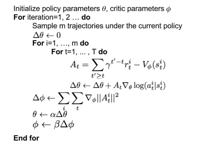
  - lastly, train critic parameters $\phi$; enforce to learn this value function, which is going to be just minimizing this advantage function and this will encourage it to be closer to the Bellman Equation
  - basically, iterating between learning and optimizing policy function and critic function, and update the gradients and repeat this process

REINFORCE in action

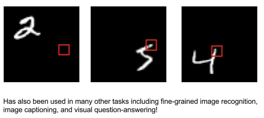
Recurrent Attention Model (RAM)

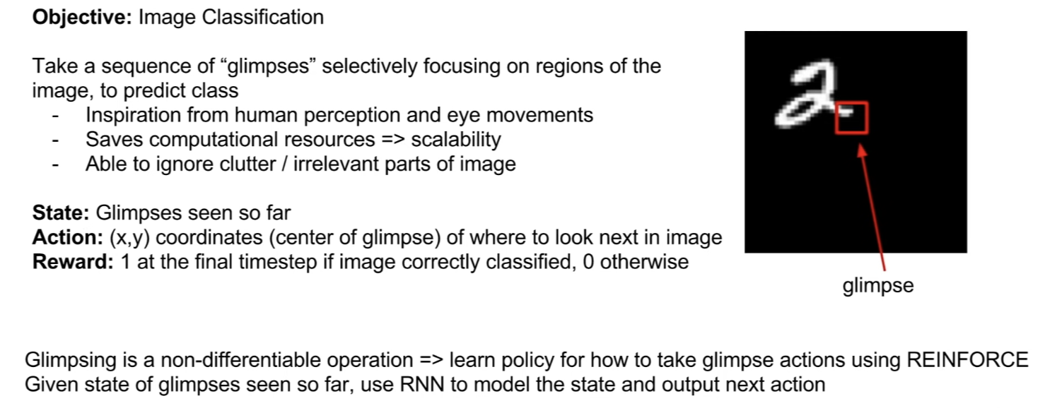
• a model also referred to as hard attention
• goal is to still predict the image class, but do this by taking a sequence of glimpses around the image
  - look at local regions around the image and selectively focus on these parts and build up information as you're looking around

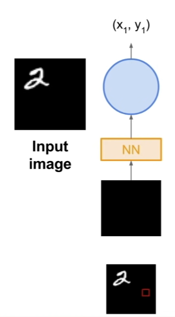
• take an input image and take a glimpse(red box)
• pass what we've seen so far into some neural network
  - we also hae to integrate glimpses we've seen so far, using a recurrent network
• output (x,y) coordinates of where to see next
  - in practice, we want to output a distribution over actions, so it will be a Gaussian distribution and we'll output the mean

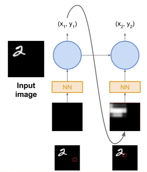
• sample a specific x, y location from action distribution and put this in to extract the next glimpse location
  - what we want to do is to look at the relevant parts of the image that are useful for classification
• pass this through neural network layers
• also pass this through a recurrent network that's taking this input as well as previous hidden state
  - this represents policy
  • use this to output distribution for the next location for glimpse

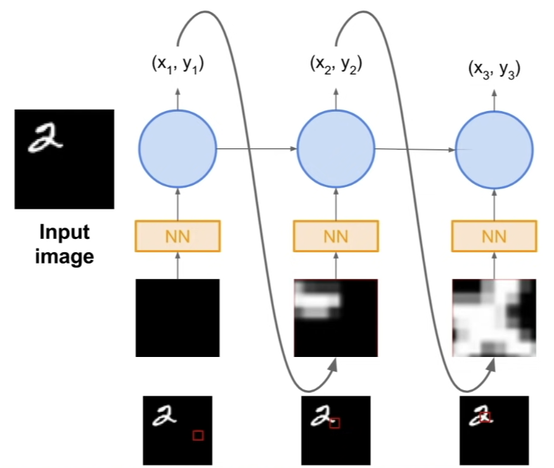
• keep doing this

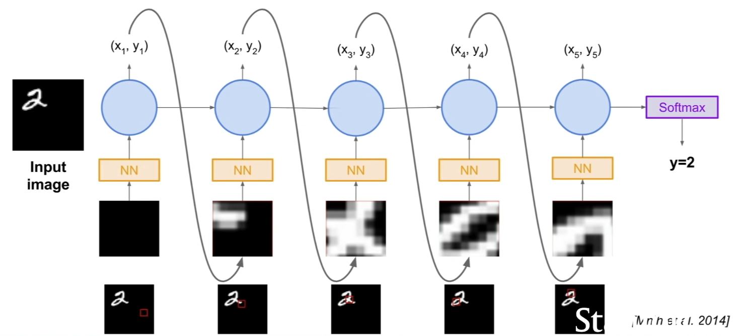
• at the final time step, since we want to do classification, we have Sofmax layer that will produce a distribution of probabilities for each class
  - here, the max class was 2

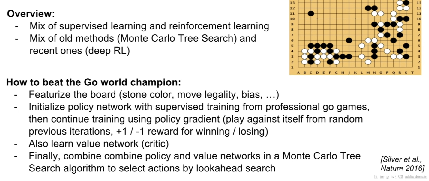
More policy gradients: AlphaGo

Summary

• Policy gradients: very general but suffer from high variacne so requires a lot of samples. Challenge: sample-efficiency
  - directly taking gradients descent or ascent on policy parameters
• Q-learning: does not always work but when it works, usually more sample-efficient. Challenge: exploration
• Guarantees:
  - Policy Gradients: Converges to a local minima of $J(\theta)$, often good enough!
  • Q-learning: Zero guarantees since you are approximating Bellman equation with a complicated function approximator