히스토그램
library(ggplot2)
library(dplyr)
df = read.csv('student_info.csv')
데이터프레임의 형태, 컬럼 형식 확인
str(df)

ggplot(df, aes(x=weight)) + geom_histogram(binwidth = 1)
ggplot(df, aes(x=weight)) + geom_histogram(binwidth = 5)
ggplot(df, aes(x=weight)) + geom_histogram(binwidth = 1, color = 'black, fill = 'gray')
ggplot(df, aes(x=weight)) + geom_histogram(binwidth = 1, color = 'black', fill = 'gray') + geom_vline(xintercept = mean(weight), color = 'red', linetype = 'dashed', size = 1)
# 혈액형 별로 출력
ggplot(df, aes(x=weight, fill = bt)) + geom_histogram(binwidth = 5)
ggplot(df.student.info, aes(x=weight, fill = bt)) + geom_histogram(binwidth = 5, position = "dodge") + theme(legend.position = "top")
산점도
df.student.info = read.csv("student_info.csv")
str(df.student.info)
ggplot(df.student.info, aes(x=weight, y=height)) + geom_point()
ggplot(df.student.info, aes(x=weight, y=height, color=bt)) + geom_point(size = 4) + ggtitle("몸무게와 체중")
boxplot
df.student.info = read.csv("student_info.csv")
str(df.student.info)
ggplot(df.student.info, aes(y=weight)) + geom_boxplot(fill = 'steelblue')
ggplot(df.student.info, aes(y=weight, fill = bt)) + geom_boxplot()
선그리기
library(ggplot2)
help(Nile)
year <- 1871:1970
flow.river <- data.frame(Nile)
df.flow.river <- data.frame(year, Nile)
str(df.flow.river)
ggplot(df.flow.river, aes(x=year, y=Nile)) + geom_line(col = 'red')
diamonds 예제
library(ggplot2)
ggplot(data = diamonds)
ggplot(data = diamonds) + geom_histogram(aes(x=carat))
ggplot(data = diamonds, aes(x=carat)) + geom_histogram()
ggplot(data = diamonds) + geom_density(aes(x=carat), fill = 'grey50')
ggplot(data = diamonds) + geom_density(aes(x=carat), fill = 'red')

ggplot(data = diamonds, aes(x=carat, y=price)) + geom_point()
ggplot(data = diamonds) + geom_point(aes(x=carat, y=price))

g1 <- ggplot(data = diamonds, aes(x=carat, y=price))
g2 <- geom_point(aes(color = color))
g1 + g2

g3 <- ggplot(data = diamonds)
g4 <- geom_point(aes(x=carat, y=price, color=color))
g3+g4
실습
전국인구조사 자료(example_population_f.csv )를 이용하여 다양한 데이터 분석을 진행하세
요.
library(ggplot2)
library(dplyr)
library(ggthemes)
df <- read.csv('example_population_f.csv', header = T, fileEncoding = 'cp949', encoding = 'UTF-8')
df
str(df)
# 첫 열 제거
df <- df[,-1]
df
# df 컬럼에서 Provinces 가 충청북도, 충청남도인 행 추출
df2 <- filter(df, Provinces  == '충청북도' | Provinces  == '충청남도')
# x축은 city, y축은 인구로 barplot()
graph <- ggplot(df, aes(x=City, y=Population, fill=Provinces)) + geom_bar(stat = 'identity') +theme_wsj()

# 보기 좋게 오름차순 정렬
graph_order <- ggplot(df2, aes(x=reorder(City, Population), y=Population, fill = Provinces)) + geom_bar(stat = 'identity') + theme_wsj()
graph_order
df3 <-filter(df, SexRatio > 1, PersInHou < 2)
df
graph2 <- ggplot(df3, aes(x=City, y=SexRatio, fill = Provinces)) + geom_bar(stat='identity') + theme_wsj()
graph2
df <- read.csv('example_population_f.csv', header = T, fileEncoding = 'cp949', encoding = 'UTF-8')
df <- df[, -1]

df <- mutate(df, SexF = ifelse(SexRatio < 1, '여자비율이 높음', ifelse(SexRatio > 1, '남자비율이 높음', '남녀비율이 같음')))
df$SexF <- factor(df$SexF)
df2 <- filter(df, Provinces == '경기도')
graph <- ggplot(df2, x=City, y = SexRatio-1, fill=SexF) + geom_bar(stat = 'identity', position = 'identity') + theme_wsj()
graph
< 경기도 성비 >

df4 <-filter(df, Provinces == '서울특별시')
graph2 <- ggplot(df4, aes(x=City, y = SexRatio - 1, fill=SexF)) + geom_bar(stat = 'identity', position = 'identity')+ theme_whj
< 서울특별시 성비 >
실습
mpg 데이터를 이용하여 다음 차트를 만들어 보세요.
1. mpg데이터의 cty와 hwy 간에 어떤 관계가 있는지 알아보려고 합니다. x축은 cty, y축은
hwy로 된 산점도를 만들어 보세요.
- midwest 데이터를 이용하여 다음을 분석하세요
- midwest 데이터를 이용해 전체 인구와 아시아인 인구 간에 어떤 관계가 있는지 알아보
려고 합니다. x축은 poptotal, y축은 popasian으로 산점도를 만들어 보세요.- 그리고, 전체 인구는 50만 이하, 아시아인 인구는 1만명 이하인 지역만 산점도에 표시되
게 하세요.
- 참고 : 지수 표시를 자연수로 하려면 options(scipen = 99) vs options(scipen = 0)
mpg <- as.data.frame(ggplot2::mpg)
1. ggplot(data = mpg, aes(x=cty, y=hwy)) + geom_point()

midwest <- as.data.frame(ggplot2::midwest)
2. ggplot(data = midwest, aes(x=poptotal, y=popasian) + geom_point()
3.
# 정수 형태로 표현
options(scipen = 99)
# 지수 형태로 표현 ex) 2e + 6
options(scipen = 0)
ggplot(data = midwest, aes(x=poptotal, y=popasian) + geom_point() + xlim(0. 500000) + ylim(0,10000)
1.mpg 데이터를 이용해서 drv별 평균 hwy를 막대그래프로 표현
2. 막대 그래프의 x축은 기본적으로 알파벳 순으로 정렬
3. reorder()를 이용하여 크기순으로 정렬 가능
mpg <- as.data.frame(ggplot2::mpg)
1.
mpg_plot <- mpg %>% group_by(drv) %>% summarise(mean_hwy = mean(hwy))
3. ggplot(data = df_mpg, aes(x=reorder(drv, mean_hwy), y = mean_hwy)) + geom_col()
코드를 입력하세요mpg 데이터를 이용해서 분석하세요
1. 어떤 회사에서 생산하는 “suv” 차종의 도시 연비가 높은지 알아보려고 합니다.
“suv” 차종을 대상으로 평균 cty가 가장 높은 회사 다섯 곳을 막대 그래프로 표현
하세요. 막대는 연비가 높은 순으로 정렬하세요.
2. 자동차 중에서 어떤 class가 가장 많은지 알아보려고 합니다. 자동차 종류별 빈도
를 표현한 막대 그래프를 만들어 보세요.
1.
mpg2 <- mpg %>% filter(class = 'suv) %>% group_by(manufacturer) %>% summarise(mean_cty = mean(cty)) %>% arrange(desc(mean_cty)) %>% head(5)
ggplot(data = mpg2, aes(x=reorder(manufacturer, mean_cty), y=mean_cty)) + geom_col()
2. ggplot(data = mpg, aes(x=class))  geom_bar()
mpg 데이터를 이용해서 분석하세요
1. class가 “compact”, “subcompact”, “suv”인 자동차의 cty가 어떻게 다른지 비교해 보려고
합니다. 상자 그래프로 만들어 보세요.mpg_plot <- mpg %>% filter(class %in% c('compact', 'subcompact', 'suv') ggplot(data = mpg_plot, aes(x=class, y=cty) + geom_boxplot()
트리맵
install.packages('treemap')
library(treemap)
tree_data <- data.frame(name = c('KIM', 'LEE', 'CHOI', 'HAN'),
                        value = c(200, 300, 50, 600))
tree_data
treemap(tree_data, index = 'name', vSize = 'value', type = 'index')

tree_mpg <- as.data.frame(ggplot2::mpg)
tree_mpg <- tree_mpg[, c('manufacturer', 'model', 'hwy')]
tree_mpg
# FUN함수 ? :
tree_mpg = aggregate(hwy ~ manufacturer + model, data = tree_mpg, FUN = mean)
tree_mpg

treemap(tree_mpg, index = c('manufacturer', 'model'), vSize = 'hwy', type = 'index')
treemap(tree_mpg, index = c('manufacturer', 'model'), vSize = 'hwy', type = 'index', palatte = 'Dark2')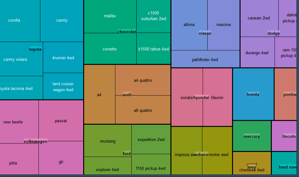

To be a DataScientist