ggplot2 패키지 특징

• 데이터를 색, 형태, 크기 등으로 달리 표시하거나 범례(레전드)를 추가하는 일이 훨씬 더 용이
• 그래프 만드는 속도 향상
• 기본 그래프 함수 30줄 가량 >> ggplot2 1줄만에 작성 가능

ggplot2 패키지 구성

• ggplot() : 사용할 데이터를 x축, y축, colour 등 그래프 요소에 매핑, aes함수 사용
  ex) ggplot(diamonds, aes(x=x, y=price, colour = clarity))
• geom() : 다양한 그래프 중 어떤 그래프 그릴지 선택, 기하객체 함수라 부름
  ex) ggplot() + geom_line(), geom_point(), geom_histogram() 등
• theme() : 많은 양의 디자인 요소를 정할 수 있는 함수

< 예제 코드 >

library(ggplot2)
빈 그래프 생성
ggplot(data= diamonds)
x축이 carat인 히스토그램 생성
ggplot(data= diamonds) + geom_histogram(aes(x=carat))
위와 동일
ggplot(data= diamonds, aes(x=carat)) + geom_histogram()
회색으로 밀도함수 생성
ggplot(data= diamonds) + geom_density(aes(x=carat), fill = "grey50") 
빨간색으로 밀도함수 생성
ggplot(data= diamonds) + geom_density(aes(x=carat), fill = "red") 
x축 carat, y축 price인 산점도 찍기
ggplot(data= diamonds,aes(x=carat, y = price)) + geom_point() 
위와 동일
ggplot(data= diamonds) + geom_point(aes(x=carat, y = price)) 

< ggplot의 경우 변수 설정으로 + 로 표현 가능!
g1 <- ggplot(data= diamonds,aes(x=carat, y = price))
g2 <- geom_point(aes(color = color))
g1 + g2
g3 <- ggplot(data= diamonds)
g4 <- geom_point(aes(x=carat, y = price, color = color))
g3 + g4

x축이 carat이고 y축이 color인 경우의 히스토그램 전부 출력(numerical만)
ggplot(diamonds, aes(x = carat)) + geom_histogram() + facet_wrap(~color)
x = 1로 고정, y = carat인 boxplot
ggplot(diamonds, aes(y = carat, x = 1)) + geom_boxplot()
x = cut, y = carat인 모든 boxplot
ggplot(diamonds, aes(y = carat, x = cut)) + geom_boxplot()
ggplot(diamonds, aes(y = carat, x = cut)) + geom_violin()
# 순서만 바꾸어 출력한 형태
ggplot(diamonds, aes(y = carat, x = cut)) + geom_point() + geom_violin()
ggplot(diamonds, aes(y = carat, x = cut)) + geom_violin() + geom_point()

ggplot2 꺾은선 그래프

• 주로 연속하는 변수를 표시하는데 사용, 범주형 자료에도 사용가능!

economics <- as.data.frame(ggplot2::economics)
economics
ggplot(economics, aes( x = date, y = pop)) + geom_line()

install.packages("lubridate")
library(lubridate)
economics$year <- year(economics$date)
economics$month <- month(economics$date , label = TRUE)
econ2000 <- economics[which(economics$year >= 2000),]
head(econ2000,5)
library(scales)

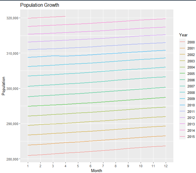
g1 <- ggplot(econ2000, aes(x = month, y = pop))
g2 <- geom_line(aes(color = factor(year), group = year)) 
g3 <- scale_color_discrete(name = "Year")
g4 <- scale_y_continuous(labels = comma)
g <- g1 + g2 + g3 + g4
g + labs( title = "Population Growth", x = "Month", y = "Population")

< 결과 >

실습 예제

mpg 데이터를 불러와 사본을 만드세요.
1. manufacturer, model, displ, drv, cty, hwy 추출
2. cty의 값을 이용하여 grade 변수 생성하세요.

• 19보다 같거나 크면 grade 변수에 H
  19보다 작고 14보다 같거나 크면 M
  그 외는 L

3. grade변수를 mpg 데이터 프레임 사본에 추가하세요.
4. grade변수가 H, M, L가 각각 몇개씩인지 카운팅하세요.
5. 한번에 cty와 hwy의 히스토그램 차트를 그려보세요.
6. grade의 변수값별로 분포를 확인(boxplot()

mpg <- as.data.frame(ggplot2::mpg)
1. mpg <- mpg %>% filter(manufacturer, model, displ, drv, cty, hwy)
mpg <- mpg[, c('manufacturer', 'model', 'displ','drv', 'cty', 'hwy')]
2,3. mpg %>% mutate(grade = ifelse(cty >= 19, 'H', ifelse(cty >= 14, 'M', 'L')))
4. table(mpg$grade)
5. par(mfrow = c(1,2))
for (i in 5:6) (
hist(mpg[,i], main = colnames(df_mpg)[i], col = 'yellow')
)
6. boxplot(mpg$cty ~ mpg$grade)

데이터 전처리

이상치 확인 및 제거

• boxplot() 이용

omit <- boxplot.stats(df.mpg$hwy)$out
df.mpg$hwy[df.mpg$hwy %in% omit] <- NA
rowSums(is.na(df.mpg))
sum(rowSums(is.na(df.mpg)) > 0)
no.outlier.df.mpg <- df.mpg[complete.cases(df.mpg),]
sum(rowSums(is.na(no.outlier.df.mpg)) > 0)

데이터 정렬

데이터 프레임 정렬

df.mpg <- data.frame(ggplot2::mpg)
order(df.mpg$hwy)
df.mpg[order(df.mpg$hwy),]
df.mpg[order(df.mpg$hwy, decreasing=T),]
df.mpg[order(df.mpg$hwy, decreasing=T, df.mpg$displ),]

데이터 집계

• aggregate()함수
  : 2차원 데이터, 데이터 그룹에 대해 평균, 합을 구하는 작업

student.list <- read.csv("example_studentlist.csv")
aggregate(student.list$weight ~student.list$bloodtype, data = student.list, FUN = mean)
aggregate(student.list$weight, by=list(student.list$bloodtype),FUN=mean)

데이터 병합

math <- data.frame(name=c("a","b","c"), math=c(70,80,90))
sci <- data.frame(name=c("a","b","d"), math=c(10,20,30))
math
sci
merge(math, sci, by=c("name"))
# left join (왼쪽은 전부 출력)
merge(math, sci, by=c("name"), all.x = T)
# right join (오른쪽은 전부 출력)
merge(math, sci, by=c("name"), all.y = T)
# outer join (전부 출력 느낌)
merge(math, sci, by=c("name"),all= T)