train_test_split()
X_train, X_test,y_train, y_test= train_test_split(iris_data.data, iris_data.target,
test_size=0.3, random_state=121)
- test_size : 전체 데이터에서 테스트 데이터 세트 크기를 얼마로 샘플링할 것인가를 결정합니다.
디폴트는 0.25, 즉 25% - train_size : 전체 데이터에서 학습용 데이터 세트 크기를 얼마로 샘플링할 것인가를 결정합니다. test_size parameter를 통상적으로 사용 train_size는 잘 사용되지 않습니다.
- shuffle : 데이터를 분리하기 전에 데이터를 미리 섞을지를 결정합니다. 디폴트는 True입니다. 데이터를 분산시켜서 좀 더 효율적인 학습 및 테스트 데이터 세트를 만드는데 사용됩니다.
- random_state : 호출할 때마다 동일한 학습/테스트용 데이터 세트를 생성하기 위해 주어지는 난수 값입니다.
train_test_split()는 호출시 무작위로 데이터를 분리하므로 random_state를 지정하지 않으면 수행할 때마다 다른 학습/테스트 용 데이터를 생성합니다.
학습/테스트 데이터 셋 분리 – train_test_split()
from sklearn.datasets import load_iris
from sklearn.tree import DecisionTreeClassifier
from sklearn.metrics import accuracy_score

iris = load_iris()
dt_clf = DecisionTreeClassifier()
train_data = iris.data
train_label = iris.target
dt_clf.fit(train_data, train_label)

# 학습 데이터 셋으로 예측 수행
pred = dt_clf.predict(train_data)
print('예측 정확도:',accuracy_score(train_label,pred))
예측 정확도: 1.0from sklearn.tree import DecisionTreeClassifier
from sklearn.metrics import accuracy_score
from sklearn.datasets import load_iris
from sklearn.model_selection import train_test_split
dt_clf = DecisionTreeClassifier( )
iris_data = load_iris()
X_train, X_test,y_train, y_test= train_test_split(iris_data.data, iris_data.target,
test_size=0.3, random_state=121)dt_clf.fit(X_train, y_train)
pred = dt_clf.predict(X_test)
print('예측 정확도: {0:.4f}'.format(accuracy_score(y_test,pred)))예측 정확도: 0.9556넘파이 ndarray 뿐만 아니라 판다스 DataFrame/Series도 train_test_split( )으로 분할 가능
import pandas as pd
iris_df = pd.DataFrame(iris_data.data, columns=iris_data.feature_names)
iris_df['target']=iris_data.target
iris_df.head()| sepal length (cm) | sepal width (cm) | petal length (cm) | petal width (cm) | target | |
|---|---|---|---|---|---|
| 0 | 5.1 | 3.5 | 1.4 | 0.2 | 0 |
| 1 | 4.9 | 3.0 | 1.4 | 0.2 | 0 |
| 2 | 4.7 | 3.2 | 1.3 | 0.2 | 0 |
| 3 | 4.6 | 3.1 | 1.5 | 0.2 | 0 |
| 4 | 5.0 | 3.6 | 1.4 | 0.2 | 0 |
ftr_df = iris_df.iloc[:, :-1]
tgt_df = iris_df.iloc[:, -1]
X_train, X_test, y_train, y_test = train_test_split(ftr_df, tgt_df,
test_size=0.3, random_state=121)print(type(X_train), type(X_test), type(y_train), type(y_test))<class 'pandas.core.frame.DataFrame'> <class 'pandas.core.frame.DataFrame'> <class 'pandas.core.series.Series'> <class 'pandas.core.series.Series'>dt_clf = DecisionTreeClassifier( )
dt_clf.fit(X_train, y_train)
pred = dt_clf.predict(X_test)
print('예측 정확도: {0:.4f}'.format(accuracy_score(y_test,pred)))
예측 정확도: 0.9556교차 검증


- K 폴드 - 단순 분할
from sklearn.tree import DecisionTreeClassifier
from sklearn.metrics import accuracy_score
from sklearn.model_selection import KFold
import numpy as np

iris = load_iris()
features = iris.data
label = iris.target
dt_clf = DecisionTreeClassifier(random_state=156)

# 5개의 폴드 세트로 분리하는 KFold 객체와 폴드 세트별 정확도를 담을 리스트 객체 생성.
kfold = KFold(n_splits=5)
cv_accuracy = []
print('붓꽃 데이터 세트 크기:',features.shape[0])
붓꽃 데이터 세트 크기: 150n_iter = 0
# KFold객체의 split( ) 호출하면 폴드 별 학습용, 검증용 테스트의 로우 인덱스를 array로 반환
for train_index, test_index in kfold.split(features):
# kfold.split( )으로 반환된 인덱스를 이용하여 학습용, 검증용 테스트 데이터 추출
X_train, X_test = features[train_index], features[test_index]
y_train, y_test = label[train_index], label[test_index]
#학습 및 예측
dt_clf.fit(X_train , y_train)
pred = dt_clf.predict(X_test)
n_iter += 1
# 반복 시 마다 정확도 측정
accuracy = np.round(accuracy_score(y_test,pred), 4)
train_size = X_train.shape[0]
test_size = X_test.shape[0]
print('\n#{0} 교차 검증 정확도 :{1}, 학습 데이터 크기: {2}, 검증 데이터 크기: {3}'
.format(n_iter, accuracy, train_size, test_size))
print('#{0} 검증 세트 인덱스:{1}'.format(n_iter,test_index))
cv_accuracy.append(accuracy)
# 개별 iteration별 정확도를 합하여 평균 정확도 계산
print('\n## 평균 검증 정확도:', np.mean(cv_accuracy)) #1 교차 검증 정확도 :1.0, 학습 데이터 크기: 120, 검증 데이터 크기: 30
#1 검증 세트 인덱스:[ 0 1 2 3 4 5 6 7 8 9 10 11 12 13 14 15 16 17 18 19 20 21 22 23
24 25 26 27 28 29]
#2 교차 검증 정확도 :0.9667, 학습 데이터 크기: 120, 검증 데이터 크기: 30
#2 검증 세트 인덱스:[30 31 32 33 34 35 36 37 38 39 40 41 42 43 44 45 46 47 48 49 50 51 52 53
54 55 56 57 58 59]
#3 교차 검증 정확도 :0.8667, 학습 데이터 크기: 120, 검증 데이터 크기: 30
#3 검증 세트 인덱스:[60 61 62 63 64 65 66 67 68 69 70 71 72 73 74 75 76 77 78 79 80 81 82 83
84 85 86 87 88 89]
#4 교차 검증 정확도 :0.9333, 학습 데이터 크기: 120, 검증 데이터 크기: 30
#4 검증 세트 인덱스:[ 90 91 92 93 94 95 96 97 98 99 100 101 102 103 104 105 106 107
108 109 110 111 112 113 114 115 116 117 118 119]
#5 교차 검증 정확도 :0.7333, 학습 데이터 크기: 120, 검증 데이터 크기: 30
#5 검증 세트 인덱스:[120 121 122 123 124 125 126 127 128 129 130 131 132 133 134 135 136 137
138 139 140 141 142 143 144 145 146 147 148 149]
## 평균 검증 정확도: 0.9- Stratified K 폴드 - 레이블(타겟) 분포를 고려한 분할
import pandas as pd

iris = load_iris()

iris_df = pd.DataFrame(data=iris.data, columns=iris.feature_names)
iris_df['label']=iris.target
iris_df['label'].value_counts()
0    50
1    50
2    50
Name: label, dtype: int64
kfold = KFold(n_splits=3)
# kfold.split(X)는 폴드 세트를 3번 반복할 때마다 달라지는 학습/테스트 용 데이터 로우 인덱스 번호 반환.
n_iter =0
for train_index, test_index in kfold.split(iris_df):
n_iter += 1
label_train= iris_df['label'].iloc[train_index]
label_test= iris_df['label'].iloc[test_index]
print('## 교차 검증: {0}'.format(n_iter))
print('학습 레이블 데이터 분포:\n', label_train.value_counts())
print('검증 레이블 데이터 분포:\n', label_test.value_counts())
## 교차 검증: 1
학습 레이블 데이터 분포:
 1    50
2    50
Name: label, dtype: int64
검증 레이블 데이터 분포:
 0    50
Name: label, dtype: int64
## 교차 검증: 2
학습 레이블 데이터 분포:
 0    50
2    50
Name: label, dtype: int64
검증 레이블 데이터 분포:
 1    50
Name: label, dtype: int64
## 교차 검증: 3
학습 레이블 데이터 분포:
 0    50
1    50
Name: label, dtype: int64
검증 레이블 데이터 분포:
 2    50
Name: label, dtype: int64
from sklearn.model_selection import StratifiedKFold
skf = StratifiedKFold(n_splits=3)
n_iter=0
for train_index, test_index in skf.split(iris_df, iris_df['label']):
n_iter += 1
label_train= iris_df['label'].iloc[train_index]
label_test= iris_df['label'].iloc[test_index]
print('## 교차 검증: {0}'.format(n_iter))
print('학습 레이블 데이터 분포:\n', label_train.value_counts())
print('검증 레이블 데이터 분포:\n', label_test.value_counts())## 교차 검증: 1
학습 레이블 데이터 분포:
2 34
0 33
1 33
Name: label, dtype: int64
검증 레이블 데이터 분포:
0 17
1 17
2 16
Name: label, dtype: int64
## 교차 검증: 2
학습 레이블 데이터 분포:
1 34
0 33
2 33
Name: label, dtype: int64
검증 레이블 데이터 분포:
0 17
2 17
1 16
Name: label, dtype: int64
## 교차 검증: 3
학습 레이블 데이터 분포:
0 34
1 33
2 33
Name: label, dtype: int64
검증 레이블 데이터 분포:
1 17
2 17
0 16
Name: label, dtype: int64dt_clf = DecisionTreeClassifier(random_state=156)
skfold = StratifiedKFold(n_splits=3)
n_iter=0
cv_accuracy=[]
# StratifiedKFold의 split( ) 호출시 반드시 레이블 데이터 셋도 추가 입력 필요
for train_index, test_index in skfold.split(features, label):
# split( )으로 반환된 인덱스를 이용하여 학습용, 검증용 테스트 데이터 추출
X_train, X_test = features[train_index], features[test_index]
y_train, y_test = label[train_index], label[test_index]
#학습 및 예측
dt_clf.fit(X_train , y_train)
pred = dt_clf.predict(X_test)
# 반복 시 마다 정확도 측정
n_iter += 1
accuracy = np.round(accuracy_score(y_test,pred), 4)
train_size = X_train.shape[0]
test_size = X_test.shape[0]
print('\n#{0} 교차 검증 정확도 :{1}, 학습 데이터 크기: {2}, 검증 데이터 크기: {3}'
.format(n_iter, accuracy, train_size, test_size))
print('#{0} 검증 세트 인덱스:{1}'.format(n_iter,test_index))
cv_accuracy.append(accuracy)
# 교차 검증별 정확도 및 평균 정확도 계산
print('\n## 교차 검증별 정확도:', np.round(cv_accuracy, 4))
print('## 평균 검증 정확도:', np.mean(cv_accuracy)) #1 교차 검증 정확도 :0.98, 학습 데이터 크기: 100, 검증 데이터 크기: 50
#1 검증 세트 인덱스:[ 0 1 2 3 4 5 6 7 8 9 10 11 12 13 14 15 16 50
51 52 53 54 55 56 57 58 59 60 61 62 63 64 65 66 100 101
102 103 104 105 106 107 108 109 110 111 112 113 114 115]
#2 교차 검증 정확도 :0.94, 학습 데이터 크기: 100, 검증 데이터 크기: 50
#2 검증 세트 인덱스:[ 17 18 19 20 21 22 23 24 25 26 27 28 29 30 31 32 33 67
68 69 70 71 72 73 74 75 76 77 78 79 80 81 82 116 117 118
119 120 121 122 123 124 125 126 127 128 129 130 131 132]
#3 교차 검증 정확도 :0.98, 학습 데이터 크기: 100, 검증 데이터 크기: 50
#3 검증 세트 인덱스:[ 34 35 36 37 38 39 40 41 42 43 44 45 46 47 48 49 83 84
85 86 87 88 89 90 91 92 93 94 95 96 97 98 99 133 134 135
136 137 138 139 140 141 142 143 144 145 146 147 148 149]
## 교차 검증별 정확도: [0.98 0.94 0.98]
## 평균 검증 정확도: 0.9666666666666667- cross_val_score( )
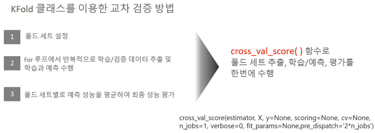
from sklearn.tree import DecisionTreeClassifier
from sklearn.model_selection import cross_val_score , cross_validate
from sklearn.datasets import load_iris
import numpy as np

iris_data = load_iris()
dt_clf = DecisionTreeClassifier(random_state=156)

data = iris_data.data
label = iris_data.target

# 성능 지표는 정확도(accuracy) , 교차 검증 세트는 3개
scores = cross_val_score(dt_clf , data , label , scoring='accuracy',cv=3)
print('교차 검증별 정확도:',np.round(scores, 4))
print('평균 검증 정확도:', np.round(np.mean(scores), 4))
교차 검증별 정확도: [0.98 0.94 0.98]
평균 검증 정확도: 0.9667- GridSearchCV
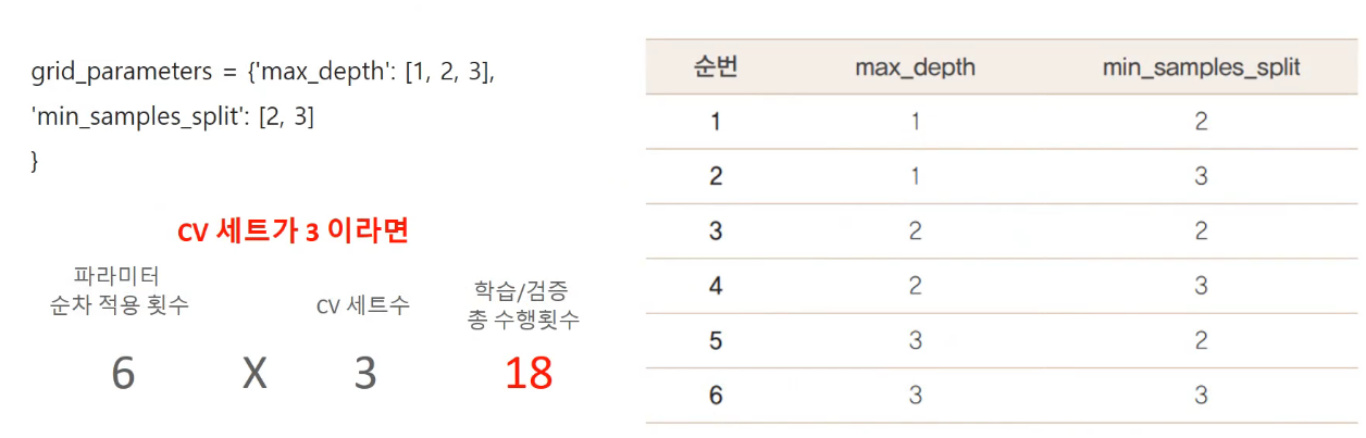
사이킷런에서는 분류 알고리즘이나 회귀 알고리즘에 사용되는 하이퍼파라미터를 순차적으로 입력해 학습을 하고 측정을 하면서 가장 좋은 파라미터를 알려준다. GridSearchCV가 없다면 max_depth 가 3일때 가장 최적의 스코어를 뽑아내는지 1일때 가장 최적인 스코어를 뽑아내는지 일일이 학습을 해야 한다. 하지만 grid 파라미터 안에서 집합을 만들고 적용하면 최적화된 파라미터를 뽑아낼 수 있다.
- GridSearchCV 클래스의 생성자 정리
- estimator : classifier, regressor, pipeline 등 가능
- param_grid : 튜닝을 위해 파라미터, 사용될 파라미터를 dictionary 형태로 만들어서 넣는다.
- scoring : 예측 성능을 측정할 평가 방법을 넣는다. 보통 accuracy 로 지정하여서 정확도로 성능 평가를 한다.
- cv : 교차 검증에서 몇개로 분할되는지 지정한다.
- refit : True가 디폴트로 True로 하면 최적의 하이퍼 파라미터를 찾아서 재학습 시킨다.
from sklearn.datasets import load_iris
from sklearn.tree import DecisionTreeClassifier
from sklearn.model_selection import GridSearchCV, train_test_split
from sklearn.metrics import accuracy_score

# 데이터를 로딩하고 학습데이타와 테스트 데이터 분리
iris = load_iris()
X_train, X_test, y_train, y_test = train_test_split(iris_data.data, iris_data.target,
                                                    test_size=0.2, random_state=121)
dtree = DecisionTreeClassifier()

### parameter 들을 dictionary 형태로 설정
parameters = {'max_depth':[1, 2, 3], 'min_samples_split':[2,3]}
import pandas as pd
# param_grid의 하이퍼 파라미터들을 3개의 train, test set fold 로 나누어서 테스트 수행 설정.
### refit=True 가 default 임. True이면 가장 좋은 파라미터 설정으로 재 학습 시킴.
grid_dtree = GridSearchCV(dtree, param_grid=parameters, cv=3, refit=True, return_train_score=True)
# 붓꽃 Train 데이터로 param_grid의 하이퍼 파라미터들을 순차적으로 학습/평가 .
grid_dtree.fit(X_train, y_train)
# GridSearchCV 결과는 cv_results_ 라는 딕셔너리로 저장됨. 이를 DataFrame으로 변환
scores_df = pd.DataFrame(grid_dtree.cv_results_)
scores_df[['params', 'mean_test_score', 'rank_test_score',
'split0_test_score', 'split1_test_score', 'split2_test_score']]| params | mean_test_score | rank_test_score | split0_test_score | split1_test_score | split2_test_score | |
|---|---|---|---|---|---|---|
| 0 | {'max_depth': 1, 'min_samples_split': 2} | 0.700000 | 5 | 0.700 | 0.7 | 0.70 |
| 1 | {'max_depth': 1, 'min_samples_split': 3} | 0.700000 | 5 | 0.700 | 0.7 | 0.70 |
| 2 | {'max_depth': 2, 'min_samples_split': 2} | 0.958333 | 3 | 0.925 | 1.0 | 0.95 |
| 3 | {'max_depth': 2, 'min_samples_split': 3} | 0.958333 | 3 | 0.925 | 1.0 | 0.95 |
| 4 | {'max_depth': 3, 'min_samples_split': 2} | 0.975000 | 1 | 0.975 | 1.0 | 0.95 |
| 5 | {'max_depth': 3, 'min_samples_split': 3} | 0.975000 | 1 | 0.975 | 1.0 | 0.95 |
grid_dtree.cv_results_{'mean_fit_time': array([0.00075221, 0.000489 , 0.00062219, 0.00023103, 0. ,
0. ]),
'std_fit_time': array([0.00018469, 0.00042131, 0.00054953, 0.00020693, 0. ,
0. ]),
'mean_score_time': array([0.00106819, 0.00041731, 0.00050243, 0.00033681, 0.00099985,
0.00100017]),
'std_score_time': array([5.20503719e-04, 3.12633361e-04, 4.11141731e-04, 4.76315584e-04,
2.24783192e-07, 1.94667955e-07]),
'param_max_depth': masked_array(data=[1, 1, 2, 2, 3, 3],
mask=[False, False, False, False, False, False],
fill_value='?',
dtype=object),
'param_min_samples_split': masked_array(data=[2, 3, 2, 3, 2, 3],
mask=[False, False, False, False, False, False],
fill_value='?',
dtype=object),
'params': [{'max_depth': 1, 'min_samples_split': 2},
{'max_depth': 1, 'min_samples_split': 3},
{'max_depth': 2, 'min_samples_split': 2},
{'max_depth': 2, 'min_samples_split': 3},
{'max_depth': 3, 'min_samples_split': 2},
{'max_depth': 3, 'min_samples_split': 3}],
'split0_test_score': array([0.7 , 0.7 , 0.925, 0.925, 0.975, 0.975]),
'split1_test_score': array([0.7, 0.7, 1. , 1. , 1. , 1. ]),
'split2_test_score': array([0.7 , 0.7 , 0.95, 0.95, 0.95, 0.95]),
'mean_test_score': array([0.7 , 0.7 , 0.95833333, 0.95833333, 0.975 ,
0.975 ]),
'std_test_score': array([1.11022302e-16, 1.11022302e-16, 3.11804782e-02, 3.11804782e-02,
2.04124145e-02, 2.04124145e-02]),
'rank_test_score': array([5, 5, 3, 3, 1, 1]),
'split0_train_score': array([0.7 , 0.7 , 0.975 , 0.975 , 0.9875, 0.9875]),
'split1_train_score': array([0.7 , 0.7 , 0.9375, 0.9375, 0.9625, 0.9625]),
'split2_train_score': array([0.7 , 0.7 , 0.9625, 0.9625, 0.9875, 0.9875]),
'mean_train_score': array([0.7 , 0.7 , 0.95833333, 0.95833333, 0.97916667,
0.97916667]),
'std_train_score': array([1.11022302e-16, 1.11022302e-16, 1.55902391e-02, 1.55902391e-02,
1.17851130e-02, 1.17851130e-02])}print('GridSearchCV 최적 파라미터:', grid_dtree.best_params_)
print('GridSearchCV 최고 정확도: {0:.4f}'.format(grid_dtree.best_score_))
# refit=True로 설정된 GridSearchCV 객체가 fit()을 수행 시 학습이 완료된 Estimator를 내포하고 있으므로 predict()를 통해 예측도 가능.
pred = grid_dtree.predict(X_test)
print('테스트 데이터 세트 정확도: {0:.4f}'.format(accuracy_score(y_test,pred)))GridSearchCV 최적 파라미터: {'max_depth': 3, 'min_samples_split': 2}
GridSearchCV 최고 정확도: 0.9750
테스트 데이터 세트 정확도: 0.9667# GridSearchCV의 refit으로 이미 학습이 된 estimator 반환
estimator = grid_dtree.best_estimator_
# GridSearchCV의 best_estimator_는 이미 최적 하이퍼 파라미터로 학습이 됨
pred = estimator.predict(X_test)
print('테스트 데이터 세트 정확도: {0:.4f}'.format(accuracy_score(y_test,pred)))테스트 데이터 세트 정확도: 0.9667
즐거운 개발공부