3-1 k-최근접 이웃 회귀

목표

• 지도 학습의 한 종류인 회귀문제 이해
• k-최근접 이웃 알고리즘 사용 농어 무게 예측하는 회귀 문제 풀기

회귀하면 또 니체죠…

---

k-최근접 이웃 회귀

• 지도학습은 크게 분류와 회귀(regression)로 나뉨
• 전 장(1-2장)에서 한게 분류
• 회귀 - 클래스 중 하나로 분류하는 것이 아닌 임의 어떤 숫자를 예측하는 문제
  • ex). 내년 경제 성장률 예측, 배달 도착 시간 예측
  • ch.3 에선 농어의 무게를 예측하는 회귀

💡

근데 회귀는 돌아온다는 뜻 아님?

회귀는 돌아오는 거야!

‘프랜시스 콜턴’이라는 통계 / 사회 학자가 키 큰 부모의 아이가 부모보다 더 크지 않다는 사실을 관찰하고 이를

평균으로 회귀한다

라고 표현했답니다. 그 후로 이렇게 굳어졌다는…

그래서 정의하면

회귀: 두 변수 사이의 상관관계를 분석하는 방법

이제 k-최근접 이웃 알고리즘이 분류와 회귀에 적용되는 방식을 알아보자

---

k-최근접 이웃 분류 알고리즘

1. 예측하려는 샘플에 가장 가까운 샘플 k개 선택
2. 샘플들의 클래스 확인해 다수 클래스를 새로운 샘플의 클래스로 예측

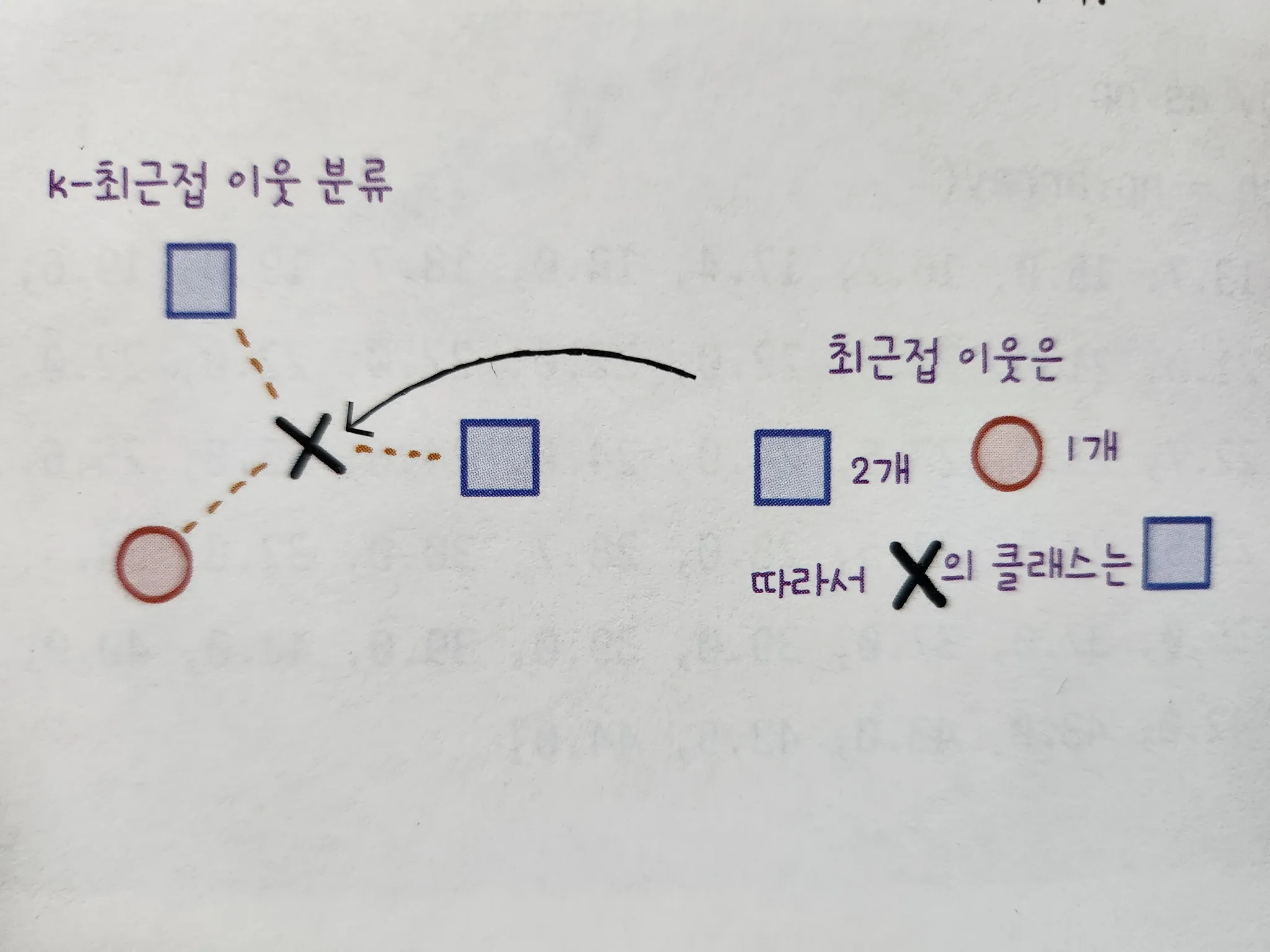
• k = 3 (샘플 3개 일 때)
• x 의 이웃에는 원1개 사각형2개 임으로 x는 네모가 된다.

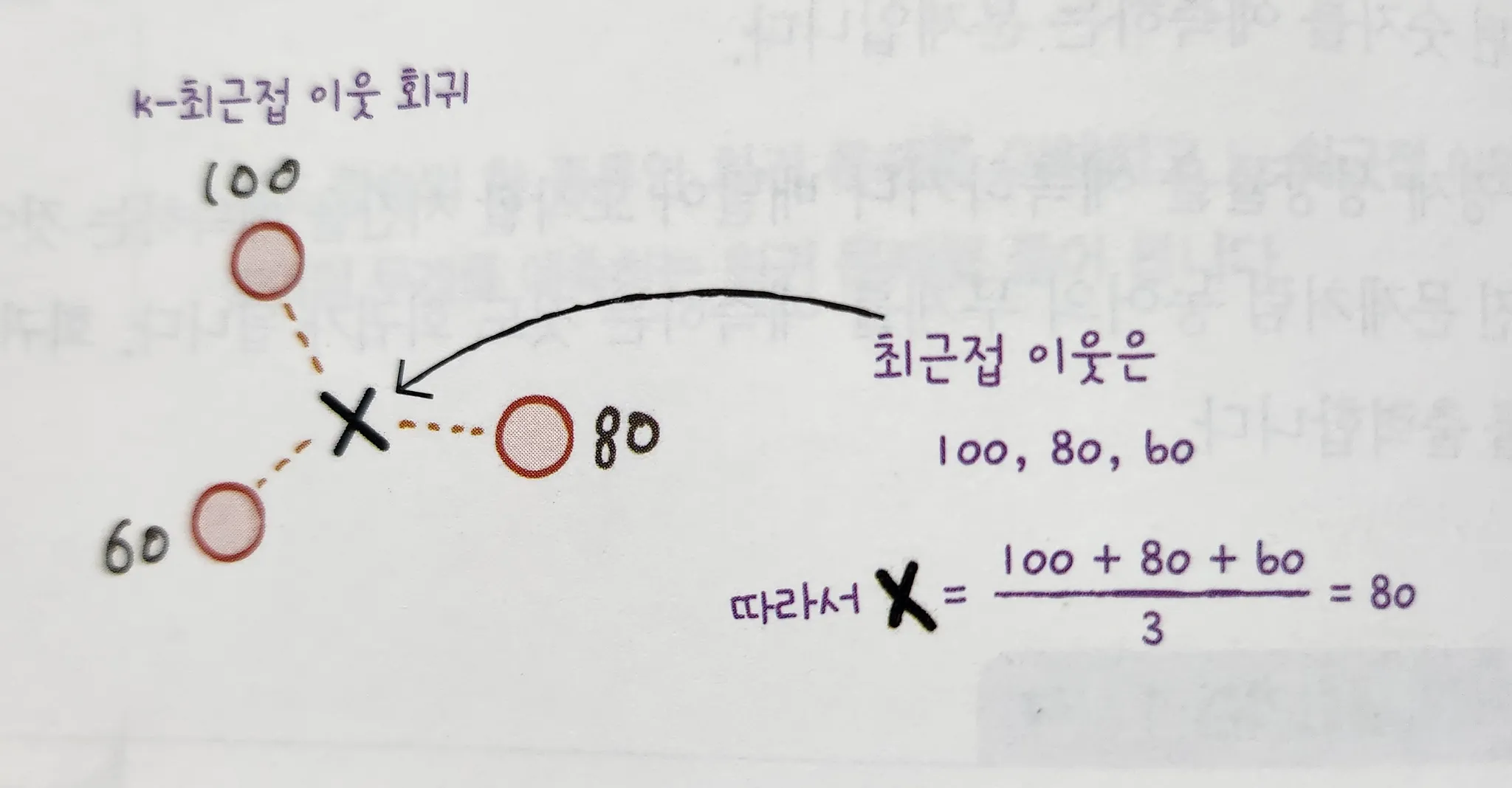
k-최근접 이웃 회귀

1. 예측할 샘플에 가장 가까운 샘플 개 선택
   • but, 회귀니까 이웃한 샘플의 타깃은 클래스가 아닌 임의의 수치(값)
2. 이웃 샘플의 수치의 평균을 구하면 샘플 x의 타깃 예측 가능

긑

---

데이터준비

• 농어 길이가 특성이고 무게가 타깃인 넘파이 배열을 준비하자

import numpy as np

perch_length = np.array(
    [8.4, 13.7, 15.0, 16.2, 17.4, 18.0, 18.7, 19.0, 19.6, 20.0,
     21.0, 21.0, 21.0, 21.3, 22.0, 22.0, 22.0, 22.0, 22.0, 22.5,
     22.5, 22.7, 23.0, 23.5, 24.0, 24.0, 24.6, 25.0, 25.6, 26.5,
     27.3, 27.5, 27.5, 27.5, 28.0, 28.7, 30.0, 32.8, 34.5, 35.0,
     36.5, 36.0, 37.0, 37.0, 39.0, 39.0, 39.0, 40.0, 40.0, 40.0,
     40.0, 42.0, 43.0, 43.0, 43.5, 44.0]
     )
perch_weight = np.array(
    [5.9, 32.0, 40.0, 51.5, 70.0, 100.0, 78.0, 80.0, 85.0, 85.0,
     110.0, 115.0, 125.0, 130.0, 120.0, 120.0, 130.0, 135.0, 110.0,
     130.0, 150.0, 145.0, 150.0, 170.0, 225.0, 145.0, 188.0, 180.0,
     197.0, 218.0, 300.0, 260.0, 265.0, 250.0, 250.0, 300.0, 320.0,
     514.0, 556.0, 840.0, 685.0, 700.0, 700.0, 690.0, 900.0, 650.0,
     820.0, 850.0, 900.0, 1015.0, 820.0, 1100.0, 1000.0, 1100.0,
     1000.0, 1000.0]
     )

• 위 데이터의 형태를 확인하기 위해 산점도를 그릴건데
  • 특성이 길이 하나 이기 때문에 특성 데이터(길이)를 x축, 타깃 데이터를 y축으로 잡는다.

import matplotlib.pyplot as plt

plt.scatter(perch_length, perch_weight)
plt.xlabel('length')
plt.ylabel('weight')
plt.show()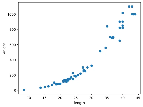

• 농어 길이가 커지면 무게도 늘어나는 관계를 찾을 수 있다.

• 이제 데이터를 훈련 세트&테스트 세트로 나누자

from sklearn.model_selection import train_test_split

train_input, test_input, train_target, test_target = train_test_split(
    perch_length, perch_weight, random_state=42)

• train_test_split 함수로 훈련/테스트 세트를 나눴다

• 결과 유지를 위해 시드는 역시 42로 고정

• 사이킷런에서 훈련 세트는 2차원 배열이여야 함

[1, 2, 3] → [[1], [2], [3]]

크기: (3, ) | (3, 1)

이렇게

💡

하나하나 변환하기 귀찮아하는 게으른 나를 위한 딸깍이 있다.

그것이 파이썬 쓰는 이유니까…

reshape

• 넘파이 배열 크기를 바꾸는 매서드
• ex). (4, ) 배열을 (2, 2)크기로 바꾸기

test_array = np.array([1,2,3,4])
print(test_array.shape)

test_array = test_array.reshape(2,2)
print(test_array.shape)

# 결과
(4,)
(2, 2)

• 이렇게 배열의 크기를 바꿀 수 있다.

!주의

• reshape() 메서드는 크기가 바뀐 새로운 배열을 반환할 때 지정한 크기가 원본 배열에 있는 원소의 개수와 다르면 에러 발생

test_array = test_array.reshape(2, 3)

# 결과
---------------------------------------------------------------------------
ValueError                                Traceback (most recent call last)
<ipython-input-9-4d70e0624945> in <cell line: 0>()
----> 1 test_array = test_array.reshape(2, 3)

ValueError: cannot reshape array of size 4 into shape (2,3)

이제 reshape를 활용하여 train_input 과 test_input 을 2차원 배열로 만들자

• 넘파이는 배열의 크기를 자동으로 지정하는 기능도 제공한다
• reshape 매서드 에서 크기에 -1 을 지정하면 나머지 원소 개수로 모두 채우라는 의미
• ex). 첫 번째 크기를 나머지 원소 개수로 채우고 두번 째 크기를 1로 하기

train_input = train_input.reshape(-1, 1)
test_input = test_input.reshape(-1, 1)
print(train_input.shape, test_input.shape)

#결과
(42, 1) (14, 1)

이제 준비한 훈련 세트로 k-최근접 이웃 알고리즘을 훈련시켜보자

---

결졍계수($R^2$)

KNeighborsRegressor

• 사이킷런에서 k-최근접 이웃 회기 알고리즘을 구현한 클래스
• 객체를 생성하고 fit으로 회귀 모델을 훈련하자

from sklearn.neighbors import KNeighborsRegressor

knr = KNeighborsRegressor()
knr.fit(train_input, train_target)

print(knr.score(test_input, test_target))

# 결과
**0.992809406101064**

점수의 의미?

• 분류의 경우 테스트 세트에 있는 샘플을 정확하게 분류한 개수의 비율(정확도, 정답 맞힌 개수 비율)

• 회귀에서는 정확한 숫자를 맞히는 것은 거의 불가능

• 회귀에서는 다르게 평가하는데 이 점수를 결정 계수라고 함($R^2$)

$R^2 = 1 - \frac{(타깃 - 예측)^2의 합}{(타깃 - 평균)^2 의 합}$

• 위에서는 0.99 정도로 좋은 값이 나왔다.
• 하지만 정확도처럼 $R^2$가 얼마나 좋은지 이해하기 어렵다.
• 타깃과 예측값 사이의 차이를 구해보면 어느정도 예측이 벗어났는지 가늠하기 좋음

mean_absolute_error

• 타깃과 예측의 절대값 오차를 평균하여 반환(사이킷런 제공 도구)

from sklearn.metrics import mean_absolute_error

# 테스트 세트 대한 예측 생성
test_prediction = knr.predict(test_input)

# 테스트 세트에 대한 평균 절대값 오차 계산
mae = mean_absolute_error(test_target, test_prediction)
print(mae)

# 결과
19.157142857142862

• 예측이 평균적으로 19g정도 타깃값과 다르다.

• 위 결과는 훈련 세트로 훈련하고 테스트 세트로 평가했다.

• 평가도 훈련세트로 하면 어떻게 될까?

• 훈련 세트의 $R^2$ 점수를 확인하자

print(knr.score(train_input, train_target))

# 결과
0.9698823289099254

• 보통 훈련 세트의 점수가 조금 더 높게 나온다(당연히 이걸로 훈련했으니까)
• 과대적합: 훈련 세트에서 점수가 좋은데 테스트 세트에서 점수가 나쁜 경우
• 과소적합: 훈련 세트보다 테스트 세트가 점수가 높거나 두 점수가 모두 너무 낮은 경우 위 경우는 테스트 세트 점수가 높으니 과소적합
  

모델을 좀 더 복잡하게 만들면 이 문제를 해결할 수 있다.

• k-최근접 이웃 알고리즘에서 모델을 복잡하게 만드는 방법
  • 이웃의 개수 k 를 줄인다.
  • 이웃을 줄이면 훈련세트에 있는 국지적인 패턴에 민감해짐(비교하는 범위가 줄어드니까)
  • 늘리면 데이터 전반의 일반적 패턴을 따를 것임
• 이웃 개수를 5에서 3으로 줄여보자

knr.n_neighbors = 3

knr.fit(train_input, train_target)
print(knr.score(train_input, train_target))

print(knr.score(test_input, test_target))

# 결과
0.9804899950518966
0.9746459963987609

k값을 줄이니 훈련 세트 $R^2$ 점수가 높아졌고

테스트 세트의 점수가 낮아져 과소적합 문제를 해결했다.

• 만약 과대적합이였다면?
• 모델을 덜 복잡하게 만들면 됨
• k값을 늘리라는 소리

키워드 정리

• 회귀: 임의의 수치를 예측하는 문제. 타깃값도 임의의 수치가 됨
• k-최근접 이웃 회귀: k-최근접 이웃 알고리즘을 사용해 문제 품
  • 가장 가까운 이웃 샘플 찾고 이 샘플들의 타깃값을 평균으로 예측
• 결졍계수($R^2$): 대표적 회귀문제 성능 측정 도구
  • 1에 가까울수록 좋고, 0에 가까우면 성능이 안좋다.
• 과대적합: 모델의 훈련 세트 성능이 테스트 세트 성능보다 훨씬 높을 때 일어남
  • 모델이 훈련 세트에 너무 집착해 데이터에 내제된 거시적 패턴 감지 불가
• 과소적합: 훈련세트와 테스트 세트 성느 모두 낮거나 테스트 세트 성능이 높을 때 발생
  • 더 복잡한 모델 사용해 훈련세트에 잘 맞는 모델 만들어서 해결

---

3-2 선형 회귀

• 책의 상황
  • 이상하게 큰 농어를 골라 무게를 예측하니 실제 무계와 너무 차이가 큰 문제 발생

k-최근접 이웃의 한계

• 우선 전에 쓴 데이터와 모델을 준비하자

import numpy as np

perch_length = np.array(
    [8.4, 13.7, 15.0, 16.2, 17.4, 18.0, 18.7, 19.0, 19.6, 20.0,
     21.0, 21.0, 21.0, 21.3, 22.0, 22.0, 22.0, 22.0, 22.0, 22.5,
     22.5, 22.7, 23.0, 23.5, 24.0, 24.0, 24.6, 25.0, 25.6, 26.5,
     27.3, 27.5, 27.5, 27.5, 28.0, 28.7, 30.0, 32.8, 34.5, 35.0,
     36.5, 36.0, 37.0, 37.0, 39.0, 39.0, 39.0, 40.0, 40.0, 40.0,
     40.0, 42.0, 43.0, 43.0, 43.5, 44.0]
     )
perch_weight = np.array(
    [5.9, 32.0, 40.0, 51.5, 70.0, 100.0, 78.0, 80.0, 85.0, 85.0,
     110.0, 115.0, 125.0, 130.0, 120.0, 120.0, 130.0, 135.0, 110.0,
     130.0, 150.0, 145.0, 150.0, 170.0, 225.0, 145.0, 188.0, 180.0,
     197.0, 218.0, 300.0, 260.0, 265.0, 250.0, 250.0, 300.0, 320.0,
     514.0, 556.0, 840.0, 685.0, 700.0, 700.0, 690.0, 900.0, 650.0,
     820.0, 850.0, 900.0, 1015.0, 820.0, 1100.0, 1000.0, 1100.0,
     1000.0, 1000.0]
     )

• 데이터를 훈련 세트와 테스트 세트로 나누자. 특성 데이터는 2차원 배열로 변환한다.

from sklearn.model_selection import train_test_split

train_input, test_input, train_target, test_target
= train_test_split(perch_length, perch_weight, random_state = 42)

train_input = train_input.reshape(-1, 1)
test_input = test_input.reshape(-1, 1)

• 이웃을 3으로하는 모델을 훈련하고 길이가 50인 농어 무게를 예측해 보자

from sklearn.neighbors import KNeighborsRegressor

knr = KNeighborsRegressor(n_neighbors = 3)
knr.fit(train_input, train_target)

print(knr.predict([[50]]))

# 결과
[1033.33333333]

• 이 길이 50cm의 농어는 1.5kg인데 예측은 더 작은 무계로 나왔다.

어째서…?

• 그 이유를 확인하기 위해 예측에 사용된 최근접 이웃을 산점도 그래프로 시각화 해보자
  • 아마 너무 길이가 길어 더 큰 개체가 표본에 없어 이웃이 오른쪽으로 치우쳐서 그러지 않을까?

import matplotlib.pyplot as plt

distances, indexes = knr.kneighbors([[50]])

plt.scatter(train_input, train_target)

# 이웃 샘플 강조
plt.scatter(train_input[indexes], train_target[indexes], marker = 'D')

# 길이 50 농어 데이터 강조
plt.scatter(50, 1033, marker = 'D')
plt.xlabel('length')
plt.ylabel('weight')
plt.show()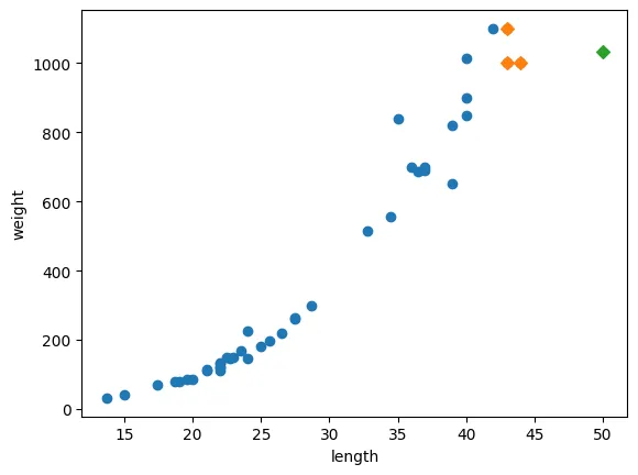

빙고

• 당연히 예측하려는 값이 혼자 끝에 있는데 평균 값이 이렇게 나올 수 밖에 없지…
  • 범위를 벗어나는 값(여기선 대략 길이가 50 넘어가는 값)을 아무라 계산해도 1033.33333333 만 나오게 된다.
• 개인적인 생각이지만 길이 대비 무게 값 관계 평균을 계산해서 점화식을 만들어 적용하는 것이 더 좋을 것 같다.

이 문제를 해결하는 다른 알고리즘이 있답니다.

---

선형 회귀

• 특성이 하나인 경우 어떤 직선을 학습하는 알고리즘
• 간단하고 성능이 뛰어남(비교적)

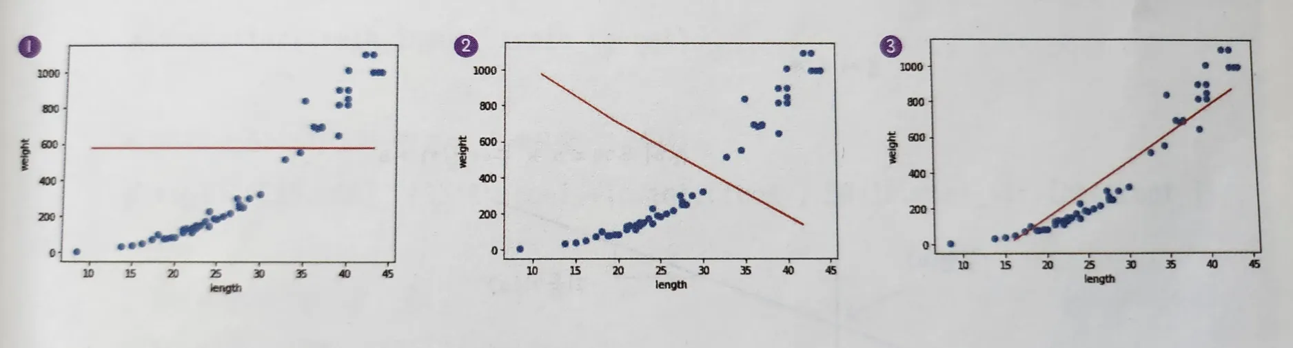
• 세 직선 중 뭐가 농어 데이터를 가장 잘 표현하는가?
• 딱 봐도 3번이다.
  • 1번 직선은 모든 농어를 하나의 무계로
  • 2번은 원래와 반대로
  • 3번이 가장 그럴싸함
• 근데 컴퓨터는 이 ‘딱 봐도’ 를 못한다. 왜? 인간이 아닌 깡통 이니까…

💡

그럼 이 직선을 인식하는 것도 구현해야 함?

• 그러기엔 난 너무 게으른 사람이다.

LinearRegression

• 선형 회귀 알고리즘을 구현한 사이킷런 제공 클래스

• 한마디로 ‘딱 봐도 이거야!’ 하는 직선을 이 깡통이 찾을 수 있게 해주는 클래스

• 마찬가지로 fit(훈련), score(평가), predict(예측) 메서드 제공

• 훈련 모델 만들고 예측해보자

from sklearn.linear_model import LinearRegression
lr = LinearRegression()

lr.fit(train_input, train_target)

print(lr.predict([[50]]))

# 결과
[1241.83860323]

• k-최근접 이웃 회귀 보다 다 더 근접하게 예측했다.

💡

LinearRegression은 어떻게 선을 그려서 예측할까?

• 다들 젊은 시절에 배웠던 직선 그리기 조건을 떠올려 보자
• 기울기와 절편이 주어져야 한다.

$y = a \times x + b$

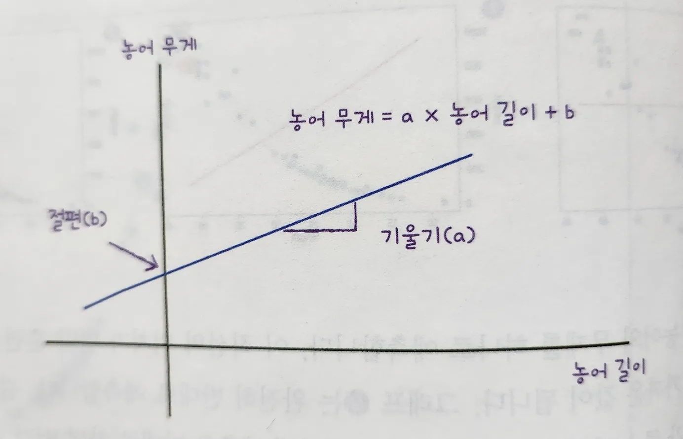
x: 농어 길이

y: 농어 무게

• x, y는 우리가 주어줬는데 a,b는??
• LinearRegression 클래스가 기울기와 절편을 스스로 잘 찾아서 객체의 coef_ 와 intercept_ 에 저장한다.
• 출력 해보자

print(lr.coef_, lr.intercept_)

# 결과
[39.01714496] -709.0186449535477

*머신러닝에선 기울기를 coefficient(계수) 또는 weight(가중치) 라고 하기도 함

• lr.coef_, lr.intercept_ 를 머신러닝 알고리즘이 찾은 값 이라는 의마로 모델 파라미터 라고 부름
• 모델 기반 학습: 최적의 모델 피라미터를 찾는 것
• 사례 기반 학습: 모델 파라미터 없이 훈련 세트를 저장 하는 게 훈련의 전부인 학습(k-최근접 이웃)

---

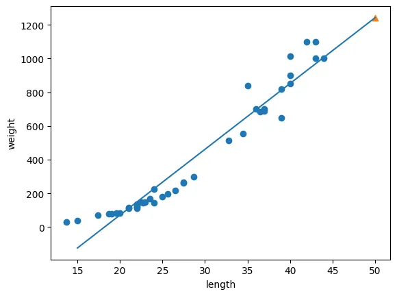
기울기와 절편이 있으니 직선을 그려보자

• 15에서 50까지 1차 방정식 그래프(직선)를 그릴거다.
• 기울기가 39, 절편이 -709이니 이걸 식에 대입만 해주면 된다
• 1539-709, 5039-709

plt.scatter(train_input, train_target)

plt.plot([15, 50], [15*lr.coef_+lr.intercept_, 50*lr.coef_+lr.intercept_])

plt.scatter(50, 1241.8, marker = '^')
plt.xlabel('length')
plt.ylabel('weight')
plt.show()

• 이 직선이 바로 선형 회귀 알고리즘이 데이터 셋에서 찾은 최적의 직선

성공

• 이제 훈련세트 범위 밖의 물고기도 예측가능하다.
• $R^2$점수도 확인해 보자

print(lr.score(train_input, train_target))
print(lr.score(test_input, test_target))

# 결과
0.939846333997604
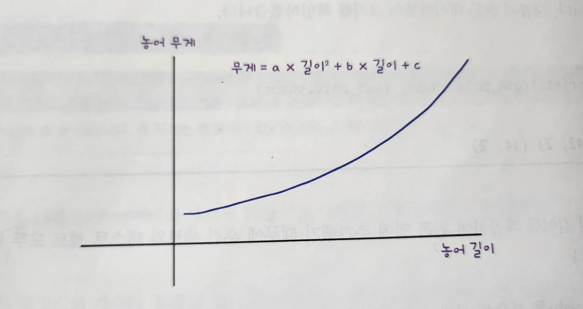
0.8247503123313558

---

다항 회귀

• 근데 직선 그래프를 좀 더 자세히 들여다 보자

  

• 이질적인 느낌이 들지 않는가?

• 직선이 우상향 이다.

• 이 직선대로 예측하면 농어의 무게가 0 이하로 내려가게 된다.

• 0g인 반물질 물고기가 현실에 존재 할 리 없는데 말이다.

• 최선의 직선 말고 곡선을 찾으면 더 좋을 것 같다.

• 곡선이 있는 그래프는 2차 방정식이 필요하겠지?

• 그럼 2차 방정식에 맞게 길이를 또 제곱 해줘야 함

• 2장에서 썼던 column_stack 함수를 쓰면 간단하게 할수있다.

• 농어의 길이를 제곱해서 원래 데이터 앞에 붙여보자
  

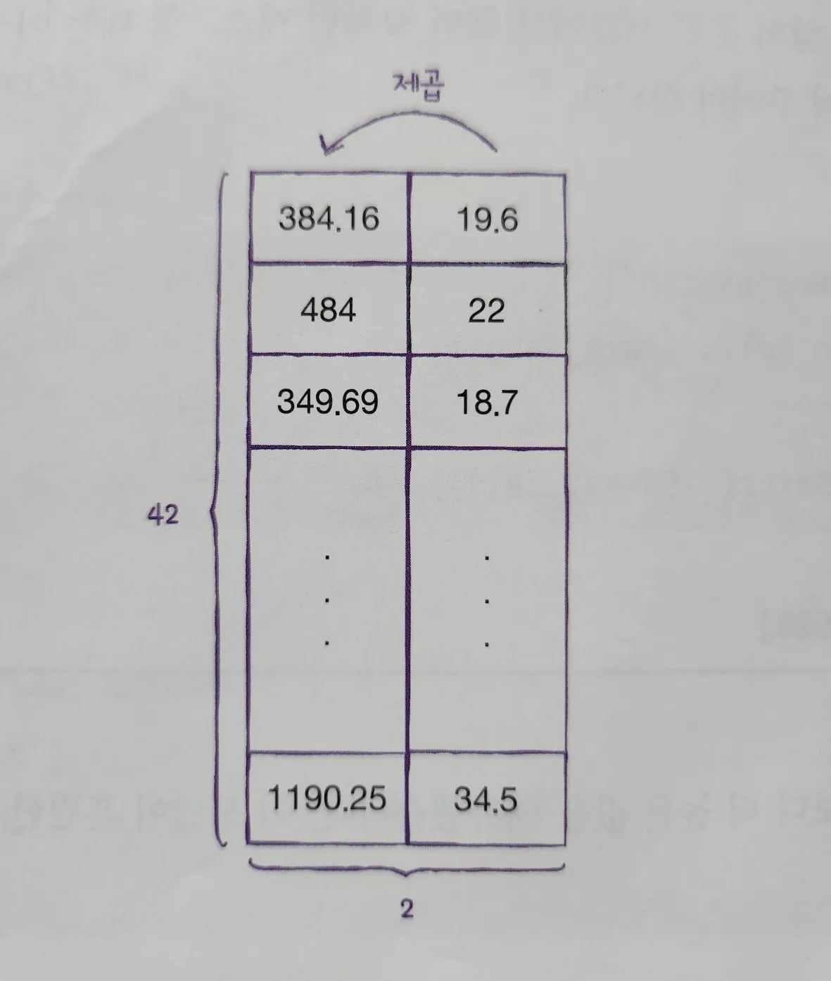
train_poly = np.column_stack((train_input ** 2, train_input))
test_poly = np.column_stack((test_input ** 2, test_input))

print(train_poly.shape, test_poly.shape)

# 결과
(42, 2) (14, 2)

• 이제 선형 회귀 모델을 다시 훈련 시킬 것인데
• 2차 방정식 그래프를 찾기 위해 제곱 항을 추가했지만 타깃 값은 그대로 사용한다.
• 목표 값 은 어떤 그래프를 훈련하던 바꿀 필요가 없다는 사실을 알아두자

lr = LinearRegression()
lr.fit(train_poly, train_target)

print(lr.predict([[50**2, 50]]))

# 결과
[1573.98423528]

• 좀 더 정답에 가까운 예측 결과다 나왔다.

• 이 모델이 훈련한 계수와 절편을 출력해 보자

print(lr.coef_, lr.intercept_)

# 결과
[  1.01433211 -21.55792498] 116.0502107827827

• 이 식을 2차방정식 그래프 식에 대입하면 모델이 학습한 그래프의 방정식을 알 수 있다.

$무계 = 1.01 \times 길이^2 - 21.6 \times 길이 + 116.05$

• 이러한 방정식을 다항식 이라 부르고
• 다항식을 사용한 선형 회귀를 다항 회귀라고 함\

---

이제 산점도에 그래프를 그려보자

point = np.arange(15, 50)

#산점도
plt.scatter(train_input, train_target)
# 2차 방정식 그래프
plt.plot(point, 1.01*point**2 - 21.6*point + 116.05)

# 50 농어 데이터
plt.scatter([50], [1574], marker = '^')
plt.xlabel('length')
plt.ylabel('weight')
plt.show()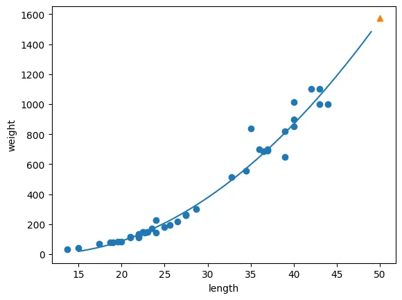

• 단순 선형 회귀보다 다항 회귀가 더 좋은 그래프가 그려졌다.

• 역시나 훈련 세트와 테스트세트의 R스퀘어 점수를 살펴보자

print(lr.score(train_poly, train_target))
print(lr.score(test_poly, test_target))

# 결과
0.9706807451768623
0.9775935108325122

• 정말 비슷하지만 테스트 점수가 쪼끔 더 높다…
• 아직 과소적합이 남아있다는 뜻