Diffusion 모델 Fine-Tuning

이 글에서는 diffusers 라이브러리를 이용한 pretrained 사용예시와 Fine-Tuning을 다뤄보고자 한다.

---

라이브러리 가져오기

import numpy as np
import torch
import torch.nn.functional as F
import torchvision
from datasets import load_dataset
from diffusers import DDIMScheduler, DDPMPipeline
from matplotlib import pyplot as plt
from PIL import Image
from torchvision import transforms
from tqdm.auto import tqdm

pretrained 모델 받기

• 모델들은 허깅페이스에 있다.

image_pipe = DDPMPipeline.from_pretrained("google/ddpm-celebahq-256")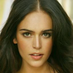
image_pipe.to(device);

• 이후로는 다음과 같이 매우 간단하게 이미지를 생성할 수 있다.

images = image_pipe().images
images[0]

---

Scheduler 받기

• scheduler에는 input x의 scale 방법과 diffusion 프로세스의 step에 따른 x와 noise 비율 계산 방법 등이 담겨 있다.
• 아래 코드를 통해 scheduler를 받을 수 있다.

scheduler = DDIMScheduler.from_pretrained("google/ddpm-celebahq-256")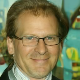
scheduler.set_timesteps(num_inference_steps=40)

• 아래 코드는 새로운 스케줄러 적용방법과 steps 조절 방법이다.

image_pipe.scheduler = scheduler
images = image_pipe(num_inference_steps=40).images
images[0]

---

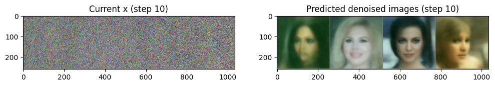
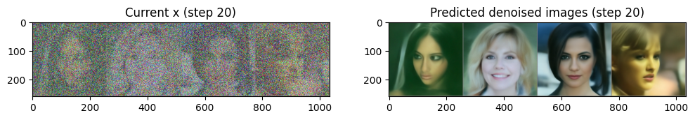
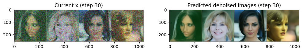
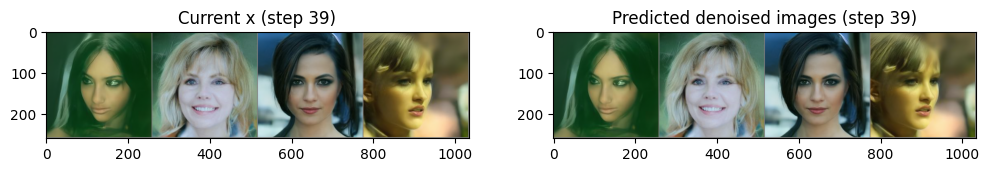
step()을 이용한 Diffusion 프로세스

• 핵심 코드 부분만 확인해보자.

# 랜덤 정규분포 : N(0, 1)
x = torch.randn(4, 3, 256, 256).to(device)

for i, t in tqdm(enumerate(scheduler.timesteps)):
    # 이미지 전처리
    model_input = scheduler.scale_model_input(x, t)

    with torch.no_grad():
        noise_pred = image_pipe.unet(model_input, t)["sample"]

    scheduler_output = scheduler.step(noise_pred, t, x)

    # Update x
    x = scheduler_output.prev_sample

• 여기서는 x의 값 범위를 (-1, 1)로 본다.
• 초기값으로 randn을 주더라도 크게 영향을 끼치지는 않는다.

x = torch.randn(4, 3, 256, 256).to(device)

• scheduler.timesteps는 다음 값들을 가지고 있다.
• 최대 steps를 1000까지 나눌 수 있을 것이다.

scheduler.timesteps

tensor([975, 950, 925, 900, 875, 850, 825, 800, 775, 750, 725, 700, 675, 650,
        625, 600, 575, 550, 525, 500, 475, 450, 425, 400, 375, 350, 325, 300,
        275, 250, 225, 200, 175, 150, 125, 100,  75,  50,  25,   0])

• U-Net에 t라는 input이 추가되었는데 model_input의 noise 강도를 알려주어 학습 및 예측에 유리하다.
• 이제 output은 denoised된 이미지가 아닌 어떤 노이즈가 씌워졌는지에 대한 output이다.

noise_pred = image_pipe.unet(model_input, t)["sample"]

• step과정에서 denoised된 pred_original_sample과
  다음 스텝에 넣을 x인 prev_sample가 계산된다.
• 다음 스텝 x의 계산식은 이전과 다르지만 t가 0에 가까워질 수록
  높은 denoise 비율을 적용한 다음 스텝 x가 계산 된다.

scheduler_output = scheduler.step(noise_pred, t, x)
x = scheduler_output.prev_sample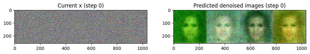

---

Fine-Tuning

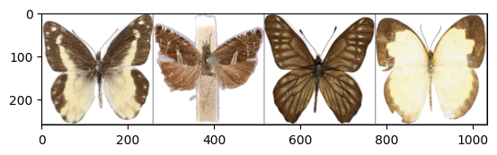
• 아래 데이터셋을 위의 사전학습된 모델에 Fine-Tuning 시켜보자.

• 이번에도 학습 프로세스의 train step 부분만 살펴보고자 한다.

lr : 1e-5
optimizer : AdamW
grad_accumulation_steps : 2

clean_images = batch["images"].to(device)
noise = torch.randn(clean_images.shape).to(device)
batch_size = clean_images.shape[0]
max_timestep = image_pipe.scheduler.num_train_timesteps

timesteps = torch.randint(0, max_timestep, (batch_size,), device=device).long()
noisy_images = image_pipe.scheduler.add_noise(clean_images, noise, timesteps)

noise_pred = image_pipe.unet(noisy_images, timesteps, return_dict=False)[0]
loss = F.mse_loss(noise_pred, noise)
loss.backward(loss)

if (step + 1) % grad_accumulation_steps == 0:
    optimizer.step()
    optimizer.zero_grad()

• 먼저 원본 이미지와 noise 이미지를 준비한다.

clean_images = batch["images"].to(device)
noise = torch.randn(clean_images.shape).to(device)

• 무작위 timesteps를 이용하여 무작위 노이즈 비율이 적용된 noisy images를 만든다.
• 수식은 아래 수식이 될 수도 있고 다른 수식이 될 수도 있다.
• x : clean_images
• n : noise
• t : timesteps
• T : max_timestep
• noisy_images : x(1-t/T) + n(t/T)

timesteps = torch.randint(0, max_timestep, (batch_size,), device=device).long()
noisy_images = image_pipe.scheduler.add_noise(clean_images, noise, timesteps)

• U-Net 출력은 어떤 노이즈가 씌워졌는지에 대한 예측이므로
  MSE loss 함수에는 noise와 noise_pred가 들어간다.

noise_pred = image_pipe.unet(noisy_images, timesteps, return_dict=False)[0]
loss = F.mse_loss(noise_pred, noise)
loss.backward(loss)

• 학습 안정성을 이유로 gradients를 몇 회 누적 후 파라미터에 적용한다.

if (step + 1) % grad_accumulation_steps == 0:
    optimizer.step()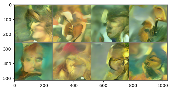
    optimizer.zero_grad()

• 학습 후 Diffusion 프로세스를 진행하여 이미지를 얻으면 다음과 같다.
• 짧은 epoch 동안만 학습하였기 때문에 괴상한 이미지가 나왔다.
• 더 긴 epoch 동안 학습 시키면 나비 모양을 확인할 수 있을 것이다.

---

Reference

• https://huggingface.co