• 유튜브 김성범[소장/인공지능공학연구소]을 보고 정리하였습니다.

Time Series Regression Model

$y_t = TR_t + \epsilon_t$

• $y_t$ : t 시점에서의 값
• $TR_t$ : t 시점에서의 trend, 모델로 잡을 수 있는 trend
• $\epsilon_t$ : t 시점에서의 error, trend로 설명하기 어려운 부분

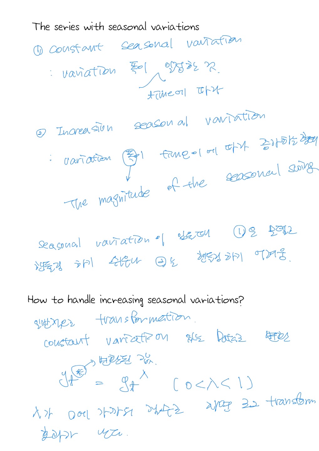
1) Trend 패턴의 종류

1. No trend : t에 따라서 변화하지 않음
   • $TR_t = \beta_0$ ⇨ Point forecast(점추정)
2. Linear trend : 증/감이 직선의 형태로 표현
   • $TR_t = \beta_0 + \beta_1t$
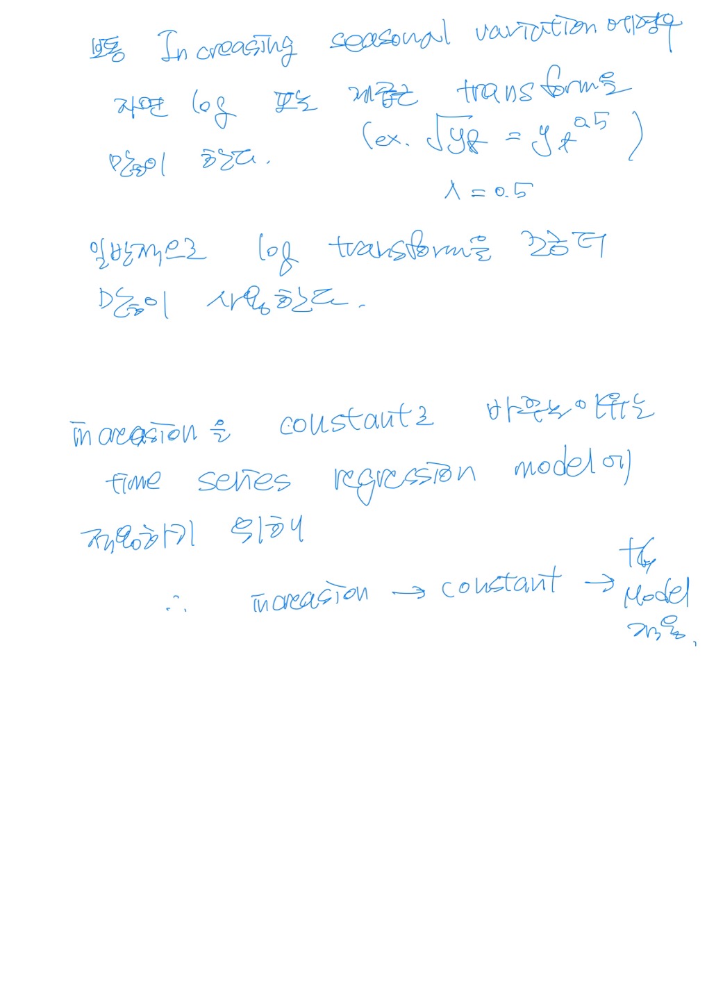
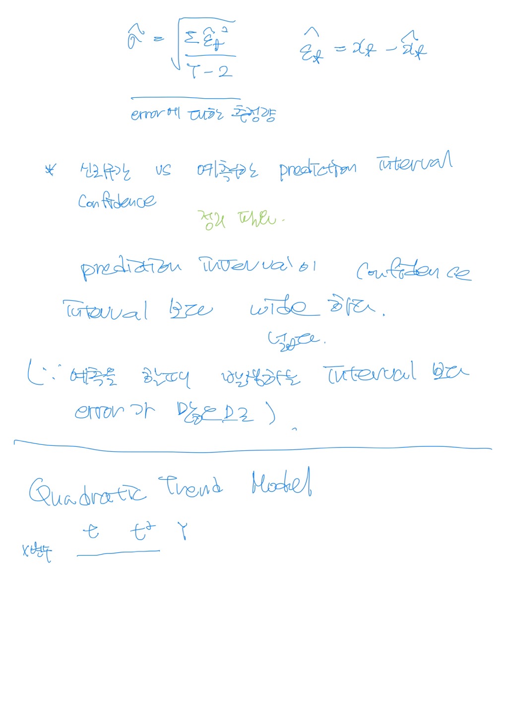
3. Quadratic(or Curvelinear) trend : 증감의 형태가 곡선으로 표현
   • $TR_t = \beta_0 + \beta_1t + \beta_2t^2$

2) Kth order polynomial time series regression models

$y_t = \beta_0 + \beta_1t + \beta_2t^2 + \cdots + \beta_kt^k + \epsilon_t, \qquad \epsilon_t \sim iid \; N(0, \sigma^2)$

• 오로지 시간(time)이 설명변수(explanantory variable)이다.
• input 변수가 단지 시간에 의해 결정된다.
• $y_t$는 오직 시간에 의해서만 결정된다.
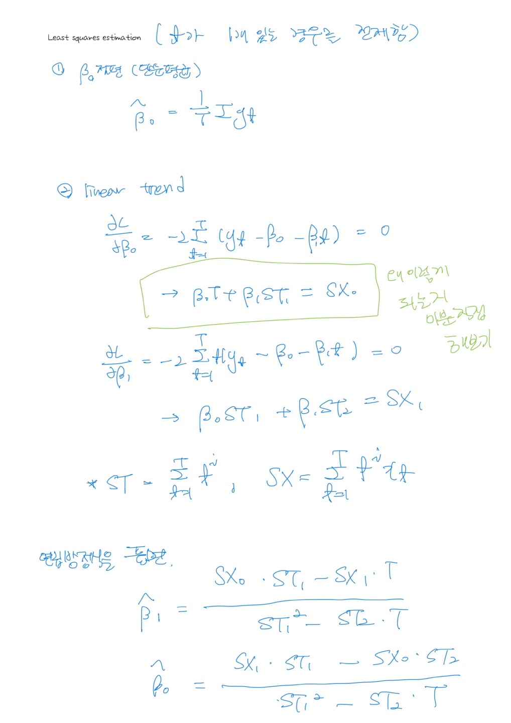
• linear trend

(1) 최소제곱법(Least-Squared Estimation)

$\hat\beta = arg \min_{\beta} L(\beta)$
$\begin{matrix} L(\beta) &=& \displaystyle\sum_{t = 1}^{T}(y_t - \beta_0 - \beta_1t - \beta_2t^2 - \cdots - \beta_kt^k)^2 \\ &=& \displaystyle\sum_{t=1}^{T}(y_t - E(y_t))^2 \\ &=& \displaystyle\sum_{t=1}^{T}(실제값 - 예측값)^2 \end{matrix}$

• $\beta$, coef 추정하는 방법
• $L(\beta)$ : loss function

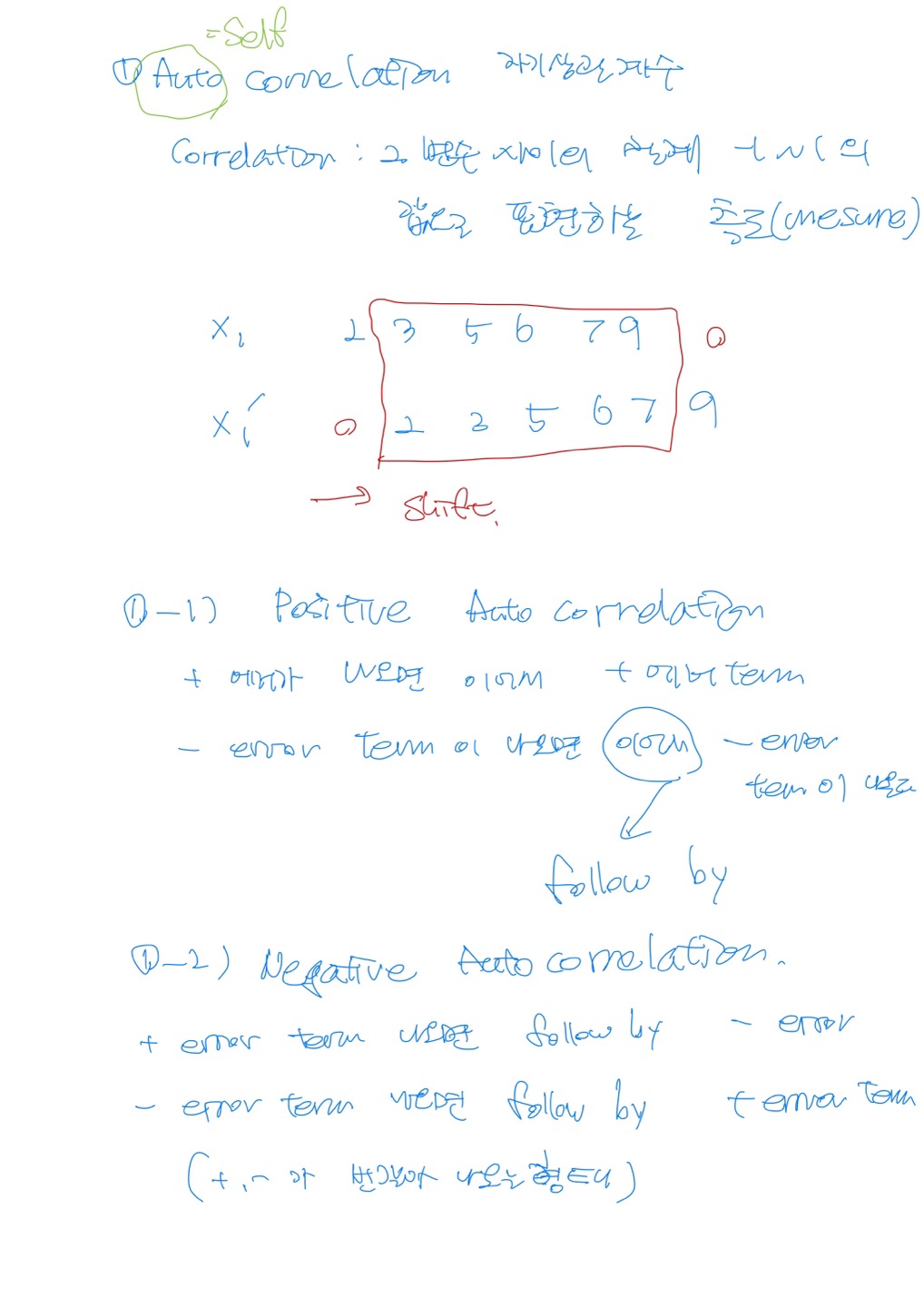
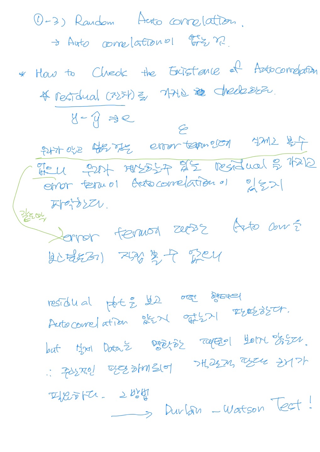
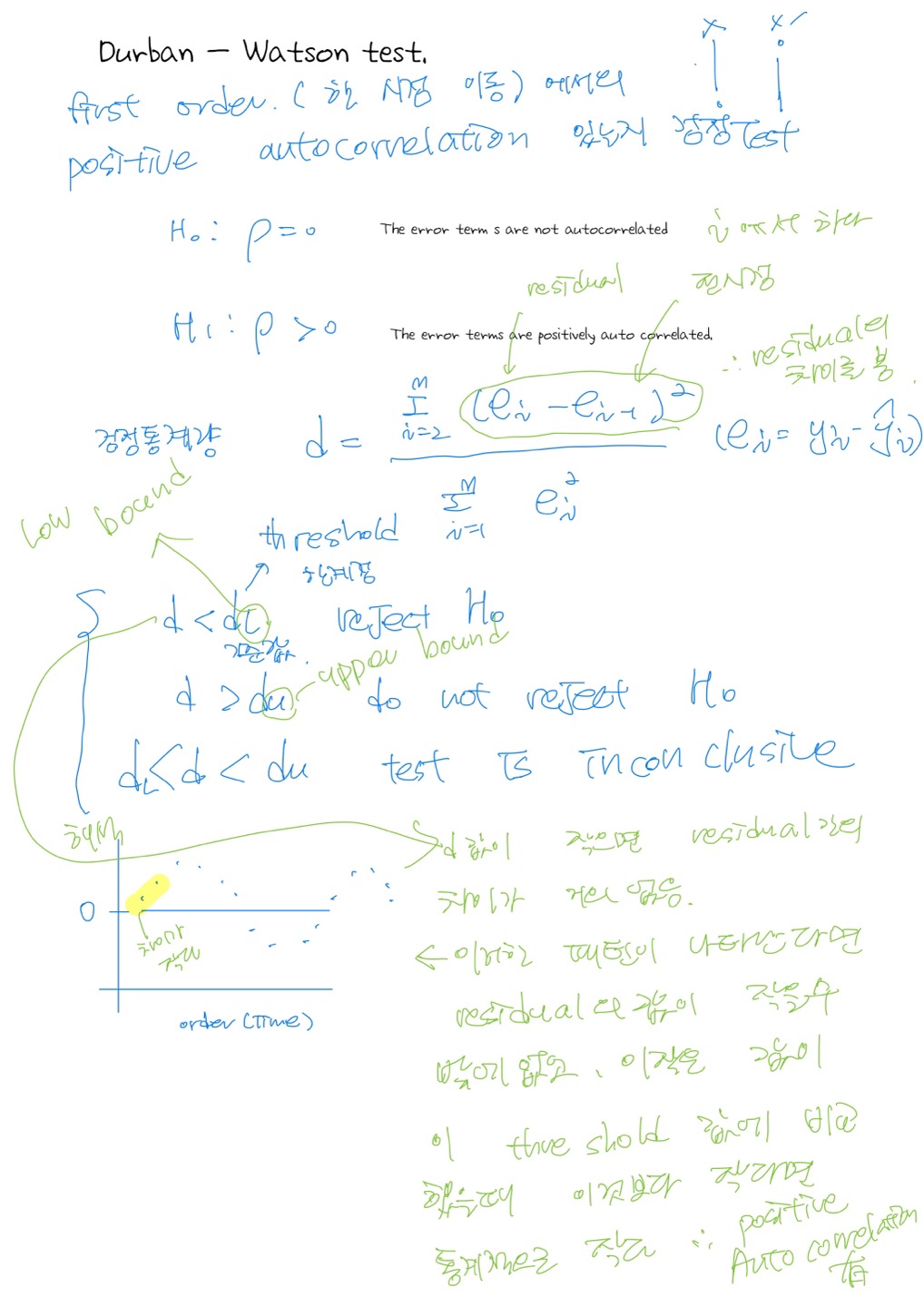
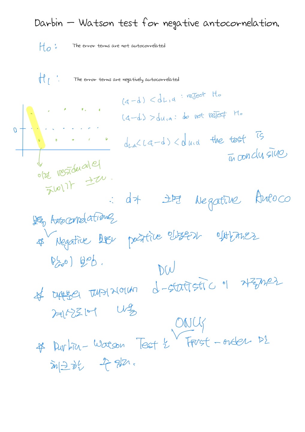
(2) Autocorrelation

• 기존 회귀분석과는 다르게 time series data는 시간에 따른 영향을 받는 데이터 이므로, $\epsilon_i$와 $\epsilon_j$는 independence하지 않기 때문에 최소제곱법을 통한 추정은 문제가 될 수 있다.
  • $Cov(\epsilon_i, \epsilon_j) = 0, \qquad (i \ne j)$라는 가정이 위배될 가능성이 多
  • Ordinary regression analysis
    • $Y_i = \beta_0 + \beta_1x_1 + \cdots + \beta_px_p + \epsilon_i$
    • x변수 : p개
    • $\epsilon_i$는 정규분포를 따르며
    • $Cov(\epsilon_i, \epsilon_j) = 0, \qquad (i \ne j)$
    • 때문에 $\epsilon_i$, \epsilon_j$는 독립이다.
• 방법의 접근이 필요하기 때문 autocorrelation을 사용한다.