
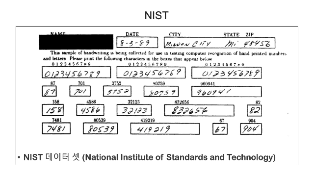
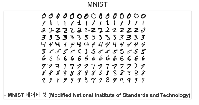
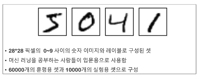
MNIST

using PCA and kNN
데이터 읽기
import pandas as pd

df_train = pd.read_csv('../ds_study/data/mnist_train.csv')
df_test = pd.read_csv('../ds_study/data/mnist_test.csv')df_train.shape, df_test.shape
train 데이터 모양
df_train.head()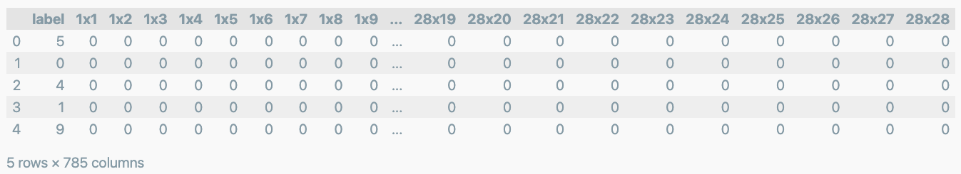
import numpy as np
np.sqrt(784)
test 데이터 모양
df_test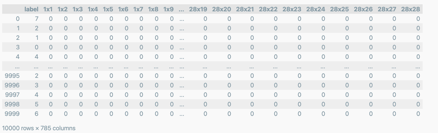
데이터 정리
import numpy as np

X_train = np.array(df_train.iloc[:,1:])
y_train = np.array(df_train['label'])

X_test = np.array(df_test.iloc[:,1:])
y_test = np.array(df_test['label'])

X_train.shape, y_train.shape, X_test.shape, y_test.shape 
데이터 확인
import random

samples  = random.choices(population=range(0,60000), k=16)
samples
random하게 16개
import matplotlib.pyplot as plt

plt.figure(figsize=(14,12))

for idx, n in enumerate(samples):
    plt.subplot(4, 4, idx+1)
    plt.imshow(X_train[n].reshape(28,28), cmap='Greys', interpolation='nearest')
    plt.title(y_train[n])

plt.show()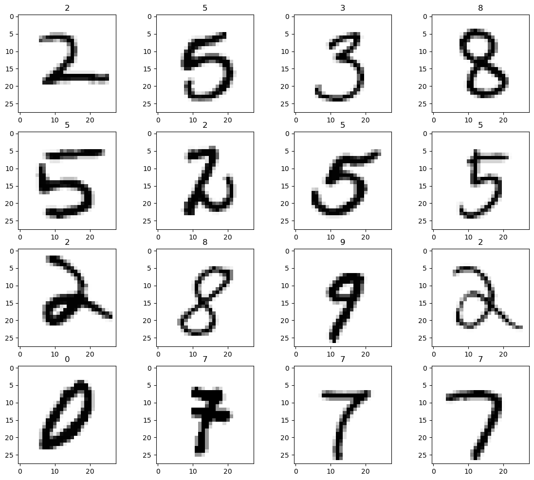
fit
from sklearn.neighbors import KNeighborsClassifier
import time

start_time = time.time()
clf = KNeighborsClassifier(n_neighbors=5)
clf.fit(X_train, y_train)
print('Fit time :', time.time() - start_time)
test 데이터 predict
from sklearn.metrics import accuracy_score

start_time = time.time()
pred = clf.predict(X_test)
print('Fit time :', time.time() - start_time)
print(accuracy_score(y_test, pred))
PCA로 차원을 줄여주자
from sklearn.pipeline import Pipeline
from sklearn.decomposition import PCA
from sklearn.model_selection import GridSearchCV, StratifiedKFold

pipe = Pipeline([
    ('pca', PCA()),
    ('clf', KNeighborsClassifier())
])

parameters = {
    'pca__n_components' : [2, 5, 10],
    'clf__n_neighbors' : [5, 10, 15]
}

kf = StratifiedKFold(n_splits=5, shuffle=True, random_state=13)
grid = GridSearchCV(pipe, parameters, cv=kf, n_jobs=-1, verbose=1)
grid.fit(X_train, y_train)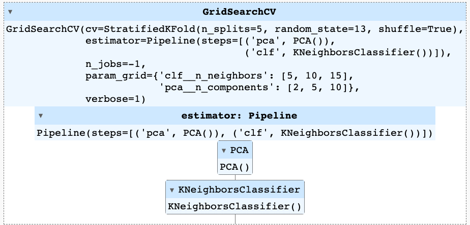
best score
grid.best_score_
grid.best_params_
단지 이정도 수준으로 약 93%의 acc가 확보된다.
pred = grid.best_estimator_.predict(X_test)

print(accuracy_score(y_test, pred))
결과 확인
def results(y_pred, y_test):
    from sklearn.metrics import classification_report, confusion_matrix
    print(classification_report(y_test, y_pred))

results(grid.predict(X_train), y_train)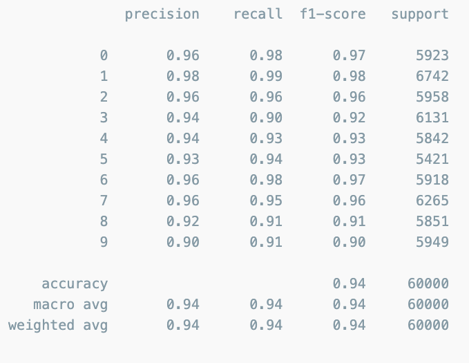
숫자를 다시 확인하고 싶다면
n = 700
plt.imshow(X_test[n].reshape(28,28), cmap='Greys', interpolation='nearest')
plt.show()

print('Answer is :', grid.best_estimator_.predict(X_test[n].reshape(1, 784)))
print('Real Label is :', y_test[n])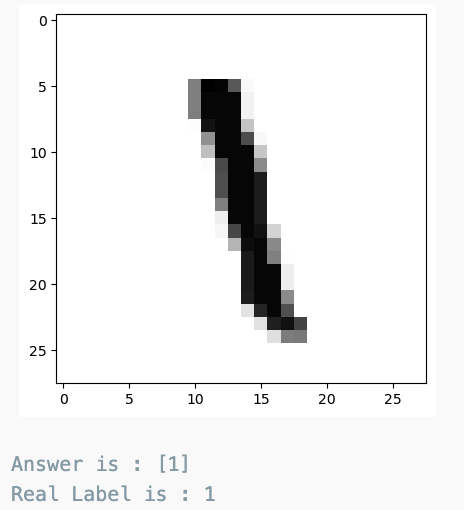
틀린 데이터를 확인
preds = grid.best_estimator_.predict(X_test)
preds
y_test
틀린 데이터를 추려서
wrong_results = X_test[y_test != preds]
samples = random.choices(population=range(0,wrong_results.shape[0]), k=16)

plt.figure(figsize=(14,12))

for idx, n in enumerate(samples):
    plt.subplot(4, 4, idx +1)
    plt.imshow(wrong_results[n].reshape(28,28), cmap='Greys')
    pred_digit = grid.best_estimator_.predict(wrong_results[n].reshape(1,784))
    plt.title(str(pred_digit))

plt.show()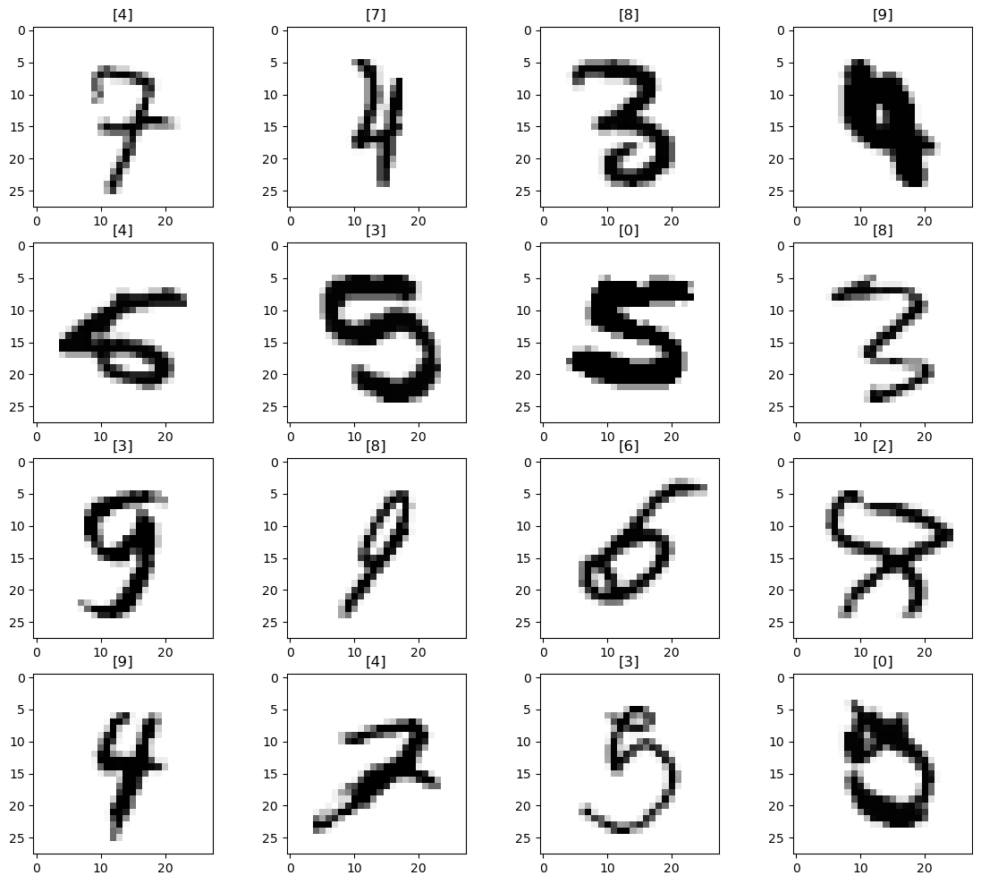

10√2 Data