

주제
게임을 진행하면서 플레이어는 게임을 진행하거나 인앱 구매를 하기 전에 잠시 기다려야 하는 게이트를 만나게 됩니다.
쿠키 캣츠의 첫 번째 게이트를 30레벨에서 40레벨로 옮긴 A/B 테스트의 결과를 분석해보았습니다. 특히 플레이어 리텐션에 미치는 영향을 분석해보았습니다.
EDA
- 라이브러리 및 데이터 불러오기
import pandas as pd
from matplotlib import pyplot as plt
import seaborn as sns

df = pd.read_csv("./data/cookie_cats.csv")- Gate_30, Gate_40 비율
a = len(df) - len(df[df["version"] == "gate_30"])
b = len(df) - len(df[df["version"] == "gate_40"])

x = [a, b]
y = ["Gate_30", "Gate_40"]

plt.figure(figsize = (12, 6))
plt.pie(x,
       labels = y,
       autopct='%.1f%%',
        startangle = 45,
       colors = plt.cm.Set2.colors)
plt.title("< Gate_30, Gate_40 비율 >")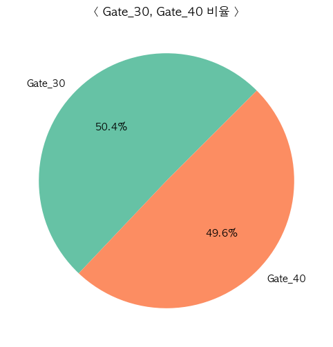
대략 50 : 50으로 잘 나눠져있는 것을 확인했습니다.
- sum_gamerounds 탐색
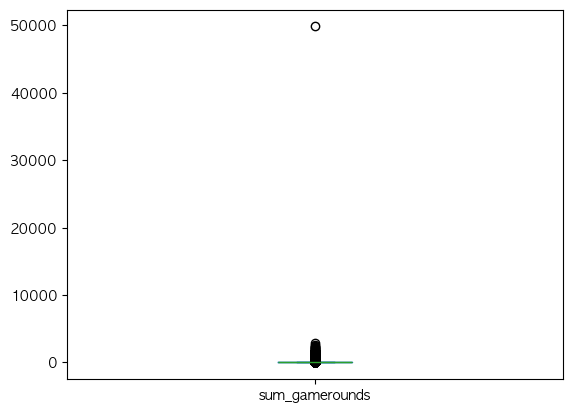
df = df.drop(df[(df["version"] == "gate_40") &
	(df["sum_gamerounds"] < 40)].index)
df = df.drop(df[(df["version"] == "gate_30") &
	(df["sum_gamerounds"] < 30)].index)
df = df.drop(df[df["sum_gamerounds"] == 49854].index)
데이터 프레임 상 눈에 띄는 이상치들만 제거후 테스트를 진행해야겠다고 판단 후 진행했습니다.
- sum_gamerounds 그룹별로 묶어서 탐색
ttmp = []

for r in df["sum_gamerounds"]:
    if r >= 30 and r < 200:
        tmp.append("A")
    elif r >= 200 and r < 400:
        tmp.append("B")
    elif r >= 400 and r < 600:
        tmp.append("C")
    elif r >= 600 and r < 800:
        tmp.append("D")
    elif r >= 800 and r < 1000:
        tmp.append("E")
    elif r >= 1000 and r < 1200:
        tmp.append("F")
    elif r >= 1200 and r < 1400:
        tmp.append("G")
    elif r >= 1400 and r < 1600:
        tmp.append("H")
    elif r >= 1600 and r < 1800:
        tmp.append("I")
    elif r >= 1800 and r < 2000:
        tmp.append("J")
    elif r >= 2000 and r < 2200:
        tmp.append("K")
    elif r >= 2200 and r < 2400:
        tmp.append("L")
    elif r >= 2400 and r < 2600:
        tmp.append("M")
    elif r >= 2600 and r < 2800:
        tmp.append("N")
    elif r >= 2800 and r < 3000:
        tmp.append("O")

df["gameround_group"] = tmp

sns.countplot(data = df,
              x = "gameround_group",
              order = df["gameround_group"].value_counts().index,
              palette = "tab10")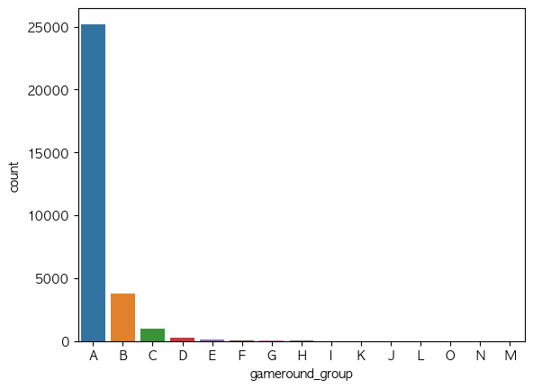
주로 200라운드 미만 그룹에서 대다수의 유저들이 몰려있는 것을 확인할 수 있었습니다.
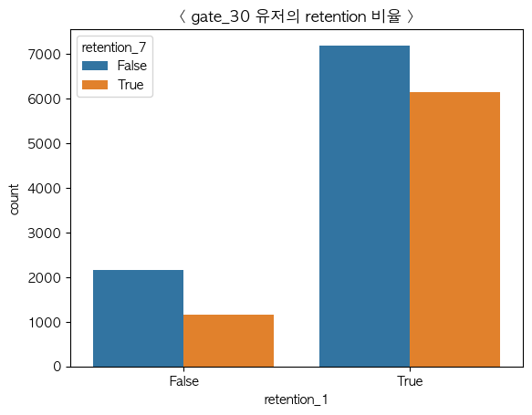
- gate_30 그룹 유저들의 retention_1, retention_7 비율 확인
plt.figure(figsize = (12, 6))

plt.subplot(1, 2, 1)
sns.countplot(data = gate_30_df,
			  x = "retention_1",
              palette = "tab10")
plt.title("< gate_30 유저의 retention_1 비율 >")

plt.subplot(1, 2, 2)
sns.countplot(data = gate_30_df,
			  x = "retention_7",
              palette = "tab10")
plt.title("< gate_30 유저의 retention_7 비율 >")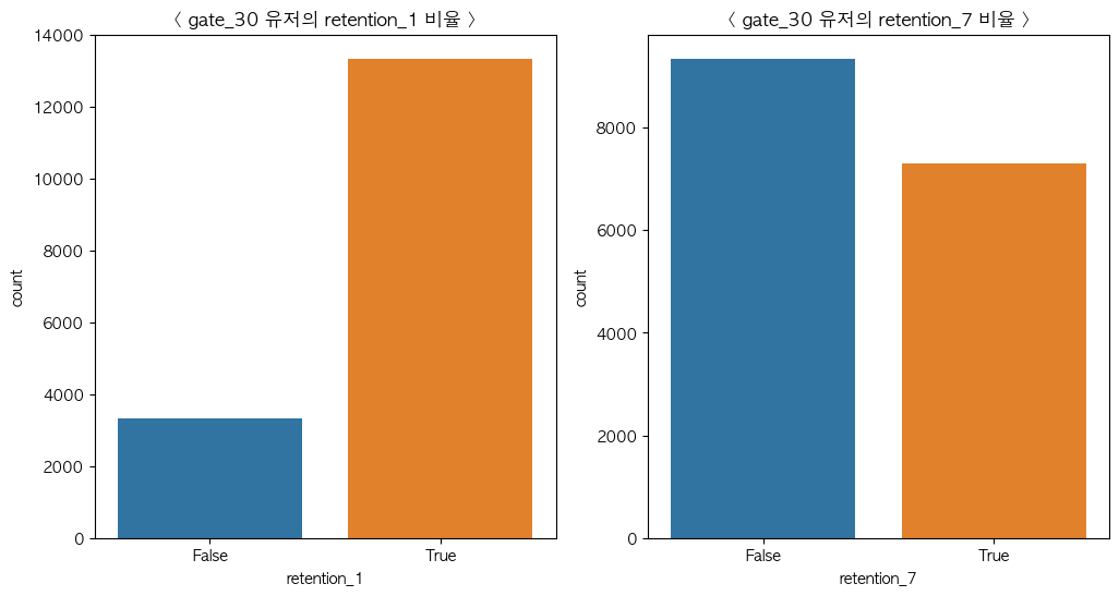
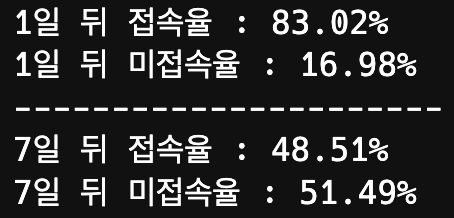
설치 1일 후 재접속율은 높으나 7일 후 재접속율은 약간 떨어지는 것을 확인할 수 있었습니다.
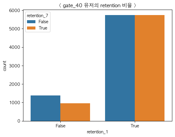
- gate_40 그룹 유저들의 retention_1, retention_7 비율 확인
plt.figure(figsize = (12, 6))

plt.subplot(1, 2, 1)
sns.countplot(data = gate_40_df,
			  x = "retention_1",
              palette = "tab10")
plt.title("< gate_40 유저의 retention_1 비율 >")

plt.subplot(1, 2, 2)
sns.countplot(data = gate_40_df,
			  x = "retention_7",
              palette = "tab10")
plt.title("< gate_40 유저의 retention_7 비율 >")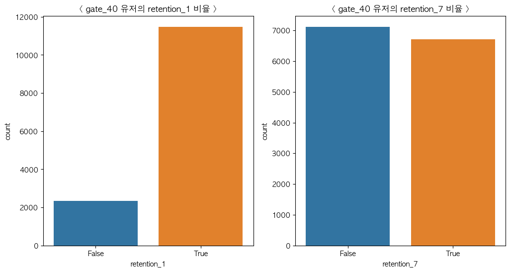
gate_30과 마찬가지로 설치 1일 후 재접속율은 높았지만 7일 후에는 약간 떨어지는 것을 확인할 수 있었지만 gate_30보다는 높은 유저가 재접속한 것을 확인할 수 있었습니다.
Test
gate_30 / gate_40 T검정
먼저 gate_30 그룹과 gate_40 그룹의 측정값의 차이를 파악하고 유의미한 차이가 있었는지 파악하기 위해
two-sample t-test 를 진행했습니다.
- 가설 설정
- 등분산 검정
gate_30_rounds = df[df["version"] == "gate_30"]["sum_gamerounds"]
gate_40_rounds = df[df["version"] == "gate_40"]["sum_gamerounds"]

_,p_value_levene = stats.levene(gate_30_rounds, gate_40_rounds)

if p_value_levene > 0.05:
    print(p_value_levene, "등분산 가정 만족")
else:
    print(p_value_levene, "이분산 가정 만족")
- Paired Sample T-Test 수행
t, p_value = stats.ttest_ind(
    a = gate_30_rounds,
    b = gate_40_rounds,
    alternative = "two-sided",
    equal_var = False
)

print(f"p-value : {p_value}")
print(f"귀무가설 기각 : {p_value < 0.05}")
귀무가설을 기각, 대립가설을 채택
따라서, gate_30 과 gate_40 그룹은 유의미한 차이가 있다.
version / retention_1 - 카이제곱검정
범주형 타입의 두 데이터가 서로 독립인지 종속인지 파악하여 서로의 데이터값의 영향을 주었는지를 파악하기 위해 카이제곱 검정을 수행했습니다.
-
가설 설정
귀무가설 : version 과 retention_1은 독립이다.
대립가설 : version 과 retention_1은 독립이 아니다. -
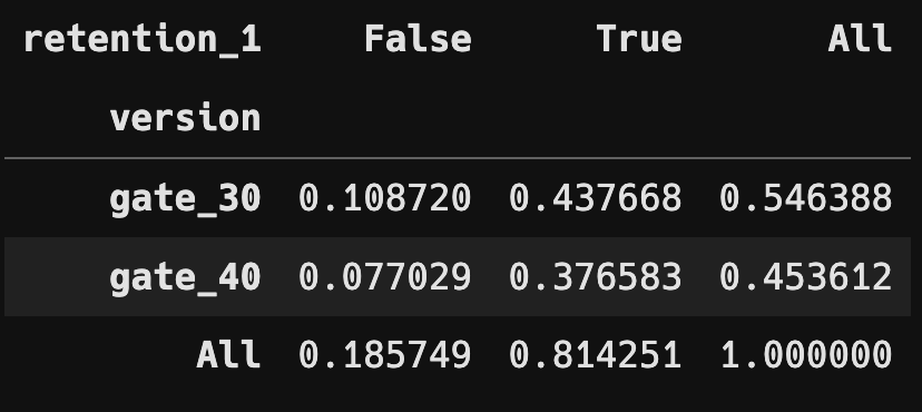
분할표 및 상대 도수 분할표
retention_1_c_table = pd.crosstab(df["version"],
								  df["retention_1"],
                                  margins = True)

retention_1_rfc_table = pd.crosstab(df["version"],
									df["retention_1"],
                                    margins = True,
                                    normalize = True)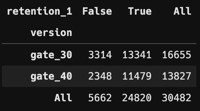
- Chi Square Test 수행
chi2_statistics, p_value, _, _ = chi2_contingency(retention_1_c_table)

print(f"Chi Squeare Statistic : {chi2_statistics}")
print(f"P-Value : {p_value}")
print(f"귀무가설 기각 : {p_value < 0.05}")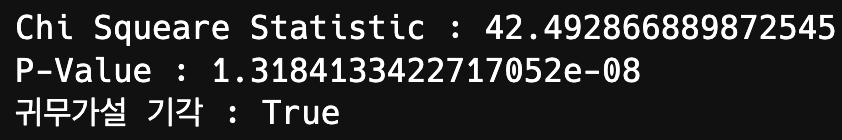
카이제곱검정으로 두 변수가 독립이 아님을 확인할 수 있었습니다.
gate_30의 제한은 1일 후 재접속율에 영향을 미칠 수 있다는 것을 확인할 수 있었습니다.
version / retention_7 - 카이제곱검정
-
가설 설정
귀무가설 : version 과 retention_7은 독립이다.
대립가설 : version 과 retention_7은 독립이 아니다. -
분할표 및 상대 도수 분할표
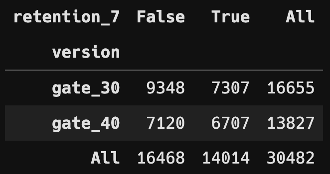
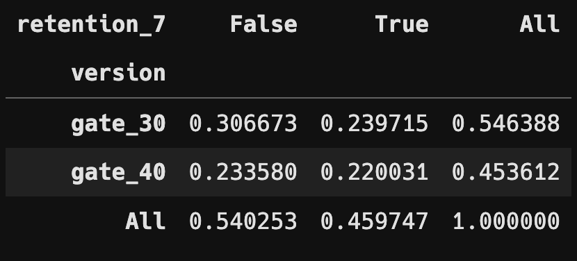
- Chi Square Test 수행
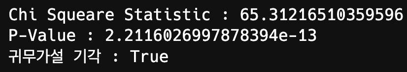
version과 retention_1, retention_7 과의 카이제곱검정을 통해 gate의 제한이 1일 및 7일 후의 재접속율에 영향을 끼친다는 것을 확인할 수 있었습니다.
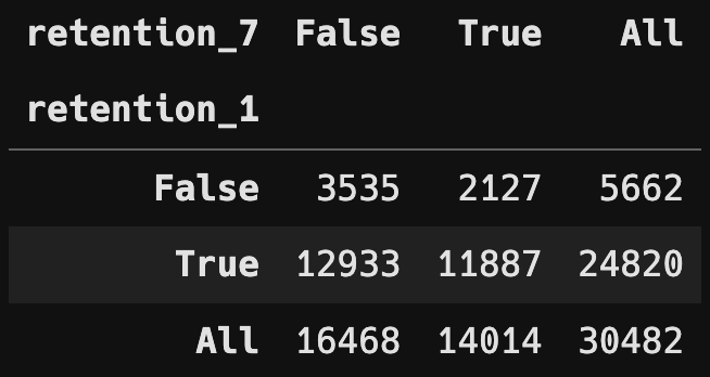
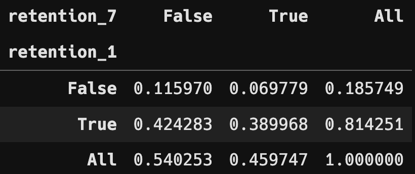
retention_1 / retention_7 - 카이제곱검정
1일 후 재접속율과 7일 후 재접속율이 서로 독립인지 종속인지를 파악해 서로에게 영향을 끼칠 수 있는 변수들인지 알고싶어 검정을 수행했습니다.
-
가설 설정
귀무가설 : retention_1 과 retention_7은 독립이다.
대립가설 : retention_1 과 retention_7은 독립이 아니다. -
분할표 및 상대 도수 분할표
- Chi Square Test 수행
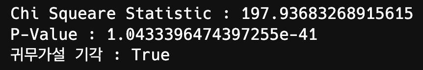
두 변수는 독립이 아니라는 것을 검정을 통해 확인했습니다.
두 변수는 영향을 주고받을 수 있는 관계라는 것을 파악할 수 있었습니다.
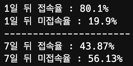
Result
- gate_30 그룹
- gate_40 그룹
-
version 과 retention 은 독립이 아닌 종속관계로 gate의 제한이 재접속율에 영향을 끼친다는 것을 카이제곱검정으로 확인했습니다.
-
gate_40을 설정한 그룹이 gate_30을 설정한 그룹보다 전체적인 미접속율이 낮은 것을 확인할 수 있었습니다.
-
30라운드는 생각 이상으로 빠르게 도달할 수 있으며 그로 인한 짧은 플레이타임으로 게임의 재미를 다 느끼기 전에 플레이가 제한될 가능성이 농후합니다.
gate를 40라운드로 미뤄 조금이나마 미접속율을 낮추는 것이 유저 경험에 도움이 될 것 같습니다.