PDP, Shap

학습내용

PDP, Shap의 장점

모델의 설명력과 복잡도는 trade off관계에 있다고 말할 수 있습니다.
즉, 모델이 복잡해질수록 성능은 좋아지지만 모델의 설명력은 떨어집니다.
PDP, Shap은 이러한 부분을 일부 해결해 줄 수 있는 방법으로 모델에 사용된 feature들이 결과에 어떻게 영향을 미치는지에 대한 정보를 줍니다.

Partial Dependence Plot(PDP)

특정 feature와 target 사이의 관계를 알기 위함, 특정 feature의 값을 변화시키며 target 값의 변화를 관찰

1. 한 특성과 target의 관계

import sklearn
import xgboost
import shap
from sklearn.model_selection import train_test_split

shap.initjs();

df, target = shap.datasets.boston()
X_train,X_test,y_train,y_test = train_test_split(df, target, test_size=0.2, random_state=2)

model = xgboost.XGBRegressor().fit(X_train, y_train)

### Draw PDP plots ###
from pdpbox.pdp import pdp_isolate, pdp_plot
import matplotlib.pyplot as plt

features = ['LSTAT', 'CRIM', 'NOX', 'RM']

for i, feature in enumerate(features):

    isolated = pdp_isolate(
        model = model,
        dataset = X_test,
        model_features = X_test.columns,
        feature = feature,
        grid_type = 'percentile', # default='percentile', or 'equal'
        num_grid_points = 100 # default=10, 한 샘플당 변화시키는 point 수
    )
    pdp_plot(isolated,
             feature_name = feature,
             plot_lines = True, #ice plots
             frac_to_plot = 10, #표시하는 ice 개수? 비율로도 줄 수 있고 정수로도 줄 수 있음, 가끔에러가 나는데 그건 왜그럴까?
             plot_pts_dist = True #rug plot 그려줌

             
             )
    plt.title(feature)
plt.show()

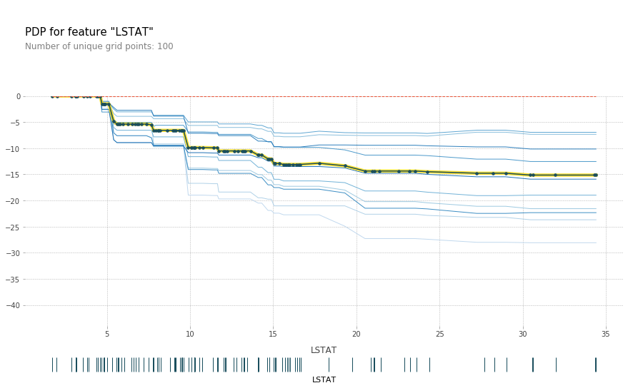
ice : 한 ICE 곡선은 하나의 관측치에 대해 관심 특성을 변화시킴에 따른 타겟값 변화 곡선이고 이 ICE들의 평균이 PDP

grid point : 한 샘플당 변화시키는 point 수

---

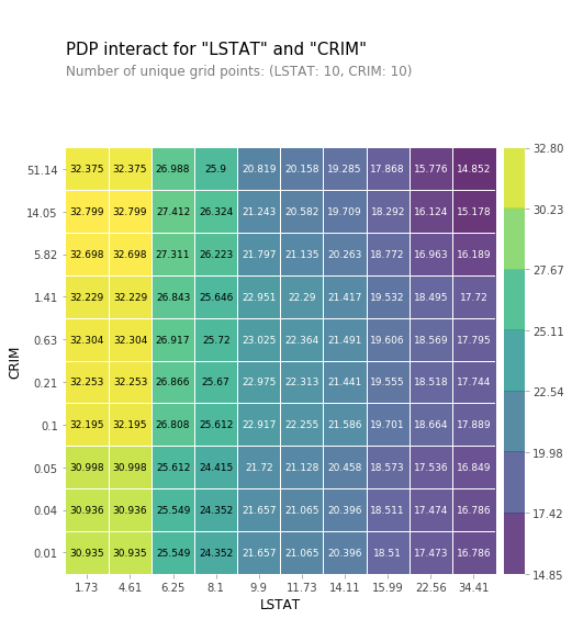
2. 두 특성과 target의 관계

• 2D로 표현

from pdpbox.pdp import pdp_interact, pdp_interact_plot

features = ['LSTAT', 'CRIM']

interaction = pdp_interact(
    model = model,
    dataset = X_test,
    model_features = X_test.columns,
    features = features
)

pdp_interact_plot(interaction,
                  plot_type = 'grid',
                  feature_names = features
                  );

• 3D로 표현

pdp = interaction.pdp.pivot_table(
    values = 'preds',
    columns = features[0],
    index = features[1]
)[::-1]

import plotly.graph_objs as go

surface = go.Surface(
    x=pdp.columns,
    y=pdp.index,
    z=pdp.values
)

layout = go.Layout(
    scene = dict(
        xaxis = dict(title=features[0]),
        yaxis = dict(title=features[1]),
        zaxis = dict(title='target')
    )
)

fig = go.Figure(surface, layout)
fig.show()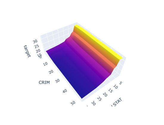

Shap

게임이론에 바탕을 두고 있으며 특정 feature를 제외했을때의 model결과와 그렇지않았을때의 model결과를 비교하여 특정 feature의 기여도를 계산하는 방식

샘플 1개에 대해서 계산된다.
, bar : permutation importance보다 더 정확하다고 할 수 있음, 이유는 밑에

1. force plot

explainer = shap.TreeExplainer(model)
shap_values = explainer.shap_values(X_test)

### Draw SHAP plots ###
shap.initjs()
shap.force_plot(
    base_value = explainer.expected_value,
    shap_values = shap_values,
    features = X_test
)

2. summary plot(분포)

shap_values = explainer.shap_values(X_train)

shap.summary_plot(
    shap_values = shap_values,
    features = X_train)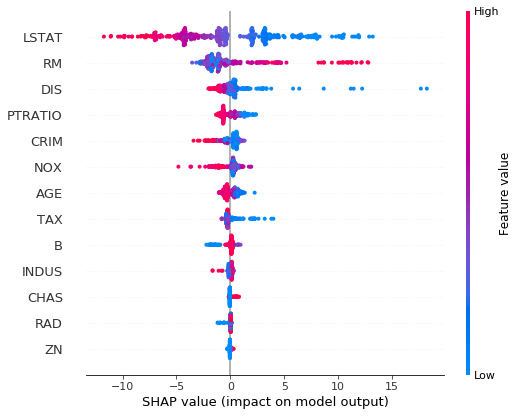

해석 : LSTAT같으 경우 feature의 값이 작아질수록 target에 양의 영향을 끼치고 있음을 알 수 있다.

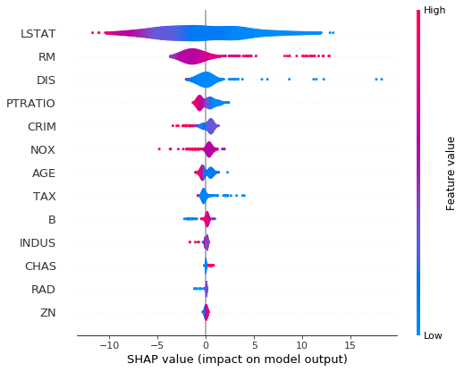
3. summary plot(바이올린)

shap.summary_plot(
    shap_values = shap_values,
    features = X_train,
    plot_type = 'violin'
)

4. summary plot(bar)

shap.summary_plot(
    shap_values,
    features = X_train,
    plot_type = 'bar'
)

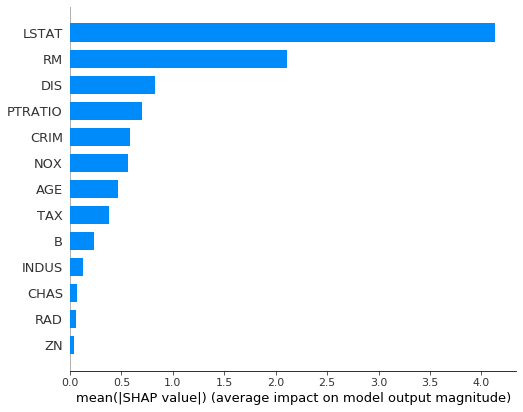
이론 상으로는 permutation importance보다 우수함

이유
1. permutation은 음의 관계에 대해서는 생각을 안함
2. permutation은 변수들이 서로 영향을 주는 경우에는 부정확함

정리

서로 관련이 있는 모든 특성들에 대한 전역적인(Global) 설명

• Feature Importances
• Drop-Column Importances
• Permutaton Importances

타겟과 관련이 있는 개별 특성들에 대한 전역적인 설명

• Partial Dependence plots

개별 관측치에 대한 지역적인(local) 설명

• Shapley Values