1. Introdution

Motivation

자세 (posture)는 “skeletal configuration of a figure”로 정의됨. - 골격 구조 [1]

이러한 골격 구조가 보다 현실적으로 느껴지게 하려면 몇 가지 constraint를 주어야 함.

• natural articulation limit → 각 골격은 일정 각도 이상 돌아갈 수 없음. (팔을 뒤로 접을 수 없는 것처럼)
• 관절들은 서로 겹칠 수 없음.
• 물리 법칙이 적용되어야 하며, 사람마다 다른 feature가 고려되어야 함. (관절의 길이, 키 등)

⇒ 이러한 요소들을 고려하여 하나의 posture를 만들었을 때, 이것이 현실적이라고 느껴질 수 있음.

모든 사람이 동일하게 갖는 general constraint (관절이 돌아갈 수 있는 최대 각도 등)을 만족해야 하지만, 사람마다 다른 특징 (키가 다른 사람들의 posture는 서로 다름)도 만족해야 함.

---

Inverse Kinematic (IK)

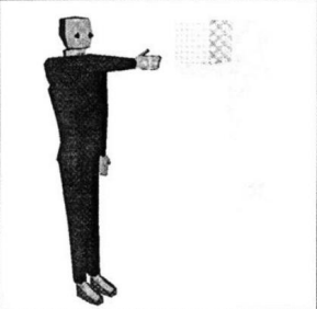
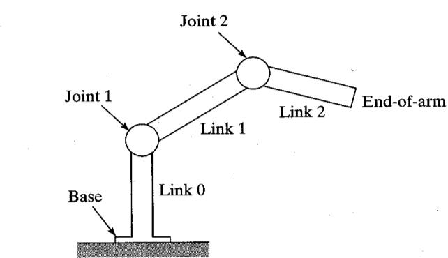
하나의 end effector (끝점)을 조작할 때, 그 자세를 만들기 위한 최적의 관절 위치를 자동으로 결정해주는 것

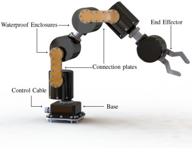
오른쪽 그림에서 로봇 팔의 end effector의 위치를 결정하는 방법은 두 가지임.

• 나머지 관절들의 각도를 모두 제공하여 end effector의 위치를 구함. → Forward Kinematic (FK)
• end effector의 위치를 옮긴 뒤 나머지 관절들이 알맞은 해 (solution)를 찾음. → Inverse Kinematic (IK)

Brief literature review

“Inverse kinematics positioning using noonlinear programming for highly articulated figures, 1994”라는 논문에서는 IK를 “Cartesian 공간에서 정의된 non-linear equation 집합의 local minimum 해”을 찾는 방식으로 해결하였음.

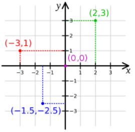
Cartesian? [2]
서로 수직인 unit vector [(1, 0), (0, 1)]로 정의된 space (걍 x, y 좌표계임)
ex) (3, 1) == $3\times \vec{e_1}+1\times \vec{e_2} \ (\vec{e_1}=(1,0), \ \vec{e_2}=(0,1))$

non-linear equation
non-linear equation은 해를 구하기가 매우 까다로움. (좌표에 따라 특징이 천차만별 → 패턴 찾기 힘듬) → non-linear를 잘 풀기 위해 사용하는 것이 딥러닝

local minimum → 완벽한 해를 구하기보다는 주어진 조건에서 최대한 에러를 줄이는 방향으로 진행

이 논문에서는 두 가지 constraint를 걸었음.

• end effector - 손
• spatial environment - 목표물

⇒ end effector (손)가 goal을 향해 뻗었을 때, 나머지 관절들의 위치를 자동으로 계산하기 위한 방법이 옛날부터 고안되었음.

---

Jacobian matrix을 사용하여 IK 문제의 linear approximation (선형 근사)를 찾음.

Jacobian matrix?
모든 값을 1차 편미분 (first-order partial derivative) 형태로 표현한 행렬. Jacobian matrix의 determinant를 Jacobian determinant라고 함.

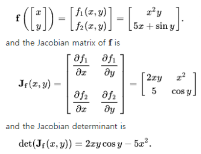
Jacobian solution을 사용하면 end effector를 움직였을 때 실시간으로 constraint를 만족하는 최적의 해를 구할 수 있음.

Jacobian solution을 구할 때에는 Jacobian inverse ($J^{-1}$)의 형태로 구하게 됨. → 생각보다 쉽지 않음. (역행렬이 존재하지 않을 수도 있고, 구하는 과정이 너무 어려울수도 있음)

→ 역행렬이 존재하지 않을 때에는 최대한 근접한 행렬을 구해야 하는데, “이걸 어떻게 함? 역행렬은 행렬의 변환인데, 근접이 존재함?”을 해결하기 위한 여러 알고리즘이 있음.

→ Jacobian Transpose, Damped Least Squares (DLS), Damped Least Squares with Singular Value Decomposition (SVD-DLS), Selectively Damped Least Squares (SDLS) 등 [3], [4], [5], [6], [7], [8]

---

Jacobian을 이용한 해법에는 몇가지 문제가 존재 → computational cost가 크고 (컴퓨터가 계산하기 힘듬), 복잡한 행렬 연산을 필요로 하며 (속도가 느려짐), singularity problem이 존재함. (해가 존재하지 않는 문제. $det(J)=0$일 때 발생 → 아무리 손을 뻗어도 목표에 도달할 수 없는 경우. 목표에 도달하지 못하더라도 어떠한 해를 나타내기는 해야 함.)

“Inverse kinematic without matrix invertion, 2008” → Jacobian Inverse를 찾지 않고도 IK를 풀 수 있는 해법 제시.

feedback loop를 사용함 → Jacobian을 사용했을 때보다 computationally efficient하고, singularity problem에 구애받지 않음.

논문의 함정 : computationally “more efficient than” ~ == 우리 기술이 얘보다는 빠른데, 사실 느림 ㅋㅅㅋ (진짜 빠르다면 real-time을 강조하거나 아예 몇 ms 정도라고 수치상으로 표현했을 것임)

Newton method를 활용한 IK 해법도 핫함. unconstrained nonlinear optimization problem을 푸는 것. (최적 해 찾기) [9]

최근에는 FTL, FABRIK과 같은 non-iterative techinique을 활용하여 IK를 해결하는 방법도 많이 나옴.

iterative → iteration을 통해 에러를 점점 줄여나가는 것. iteration의 횟수가 늘어날수록 정확한 결과가 나오겠지만 time consuming함. (시간이 오래걸림) → iteration 없이 한번에 해결하는 것이 non-iterative 방식

2. The Articulated Body Model

IK를 하기 위해서는 먼저 “데이터의 구조”를 알아야 함.

모션 데이터를 다루기 위해서는 연결된 관절마다 최대 회전 각도, 회전 평면 등의 정보가 정의되어 있어야 함.

그래픽스 어플리케이션에서 사용하는 human body는 수많은 joint들로 이루어져 있고, 이들은 서로 다른 Degree of Freedom (DoF)와 restriction (제한. 몇 도 이상 움직이면 안됨. 등등)을 가짐.

DoF → 구동 가능한 범위.

앞-뒤로만 구동 가능할 때 DoF == 1 (1개의 축)

x, y 2개의 축으로 이동 가능. DoF == 2

x, y, z축 → DoF == 3
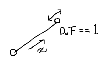
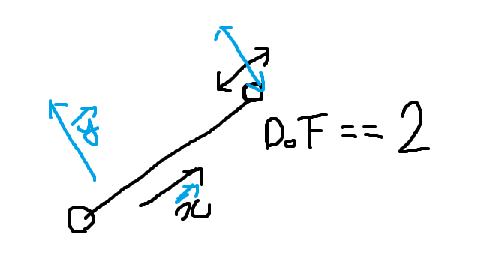
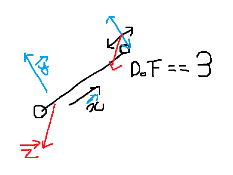
(x, y, z축 이동이 모두 가능하다는 전제 → DoF > 3)

• x, y, z축 중 한 축에 대한 회전만 가능 ⇒ DoF == 4
• 두 축에 대한 회전 가능 ⇒ DoF == 5
• 모든 축에 대한 회전이 가능함 ⇒ DoF == 6 → 우리가 상상하는 대부분의 회전이 가능한 상태

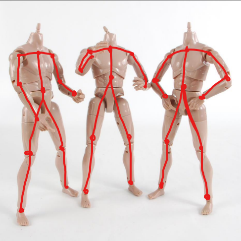
Human body modeling

인간의 몸은 강체 (rigidbody)로 이루어져 있다고 가정함. → 실제로 우리 몸은 강체가 아니기 때문에 탄성 등을 고려할 때 rigidbody는 맞지 않음. but IK에서는 그걸 고려하지 않아도 됨.

rigidbody: 강체. 딱딱한 물체라고 생각하면 됨. ↔ 유체 (fluid) : 흐를 수 있는 것.

주로 joint를 기준으로 회전 등을 정의함.

link: joint를 서로 연결함

human modeling에는 virtual body modelling이 사용됨.

잘 만들어진 모델은 실제 사람처럼 움직이도록 constraint가 잘 설정되어 있어 현실적인 모션을 보여줄 수 있음.

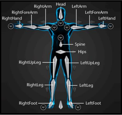
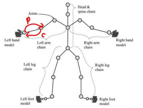
skeletal structure에서는 ⭐parent-child system⭐을 사용함. → 모든 joint들은 자신의 parent와 child를 가짐.

• child가 없는 joint들을 end-effector라고 부름.
• parent joint가 바뀌면 child joint도 이에 따라 바뀜. (parent에 맞추기 위해)
• end-effector에서부터 root까지 하나의 체인으로 이루어져 있음. (left arm chain, right leg chain 등등)
• IK에서는 체인 위주로 변화가 일어남. (체인 외의 골격은 크게 변하지 않음)
• 예외 → 중력이 작용하여 무게중심이 적용될 때 → ex. 왼쪽 다리를 들었을 때 무게중심을 유지하기 위해 오른쪽 다리가 바뀜. → 최신 ****기술에서는 물리 법칙 등을 고려하여 최적의 posture를 만드는 것을 목표로 하고 있음.

virtual body modelling. skeletal structure

---

수많은 joint를 관리하기 위해 joint에 번호를 부여하여 “i번째” joint와 같이 다룸.

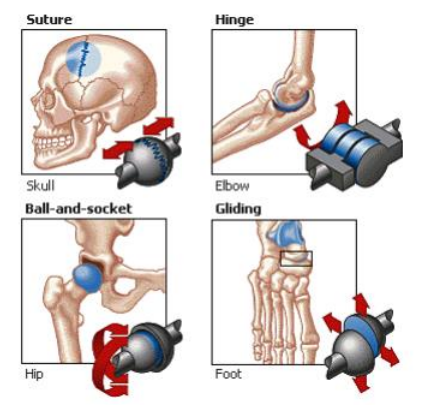
human model에 쓰이는 주요 joint는 다음과 같음.

• suture joint model (1 DoF) : 절대 열리면 안되는 fixed joint. 움직이더라도 매우 제한적으로 움직일 것. 두개골과 같은 곳에 쓰임.
• hinge joint model (1 DoF) : 가장 단순한 형태의 joint. 팔꿈치, 무릎, 손가락/발가락 등에 사용됨. 한 방향으로만 rotation이 이루어짐.
• gliding joint model (2 DoF) : 손목, 발목과 같이 보다 넓게 회전이 가능한 joint
• saddle joint model (2 DoF) : hinge나 gliding보다 자유롭게 움직일 수 있는 joint. 두 방향으로 움직일 수 있음.
• pivot joint model (2 DoF) : 목과 같은 곳에 쓰이는 joint. 좌우로 돌릴 수 있음.
• ball and socket joint model (3 DoF) : 인체에서 가장 유동적인 형태의 joint. 타원형 joint임.

Motion

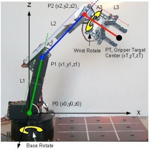
body model을 정의했으면 관절을 적절하게 translate하고 rotate해서 새로운 posture를 만들고, 이를 통해 애니메이션을 만들 수 있음.

rotational transformation & translational transformation을 사용하여 end-effector를 변화시키고, 이에 따라 연결된 체인 또한 desired position으로 이동하게 됨.

FK vs IK

• FK : position에 대한 정보를 모두 정의해주면 그에 맞는 posture가 나오는 방식.
  • input : joint angle (어떤 joint를 얼마만큼 회전시키겠다 등)
  • output : 최종 link position, orientation. end-effector의 position
• IK : end-effector의 위치를 결정하면 주변 joint를 추적하여 적절한 위치를 계산하고, 최종적으로 각 joint의 angle을 구함. (결과를 주시면 파라미터를 드립니다 ^_^)
  • input : end-effector position
  • output : joint angle

IK의 단점 → 애니메이션 등을 만들 때 디테일한 관절의 움직임을 구현하지 못할 수 있음.

---

FK problem은 unique solution이 존재함. → 주어진 input에 따라 정해진 posture가 나옴.

FK의 성공 여부는 constraint를 만족하는 결과가 나왔는지에 따라 나뉨. (constraint angle에 맞는 결과가 나오면 성공)

하지만 IK는 single solution이 존재하지 않을수도 있음.

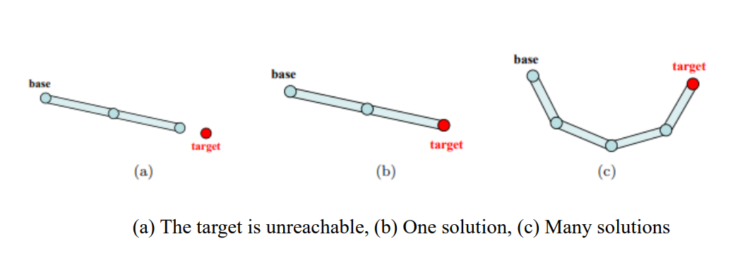
• 목표가 닿을 수 없는 곳에 있는 경우 → 해를 구할 수는 없지만, 목표에 도달하려는 움직임을 표현해야 함. → over-constrained problem
• 해가 1개 이상인 경우 → 대부분의 경우. 하나의 목표에 대해 다양한 형태의 관절이 나올 수 있음. 수많은 해 중 어떤 해를 선택해야 하지? → IK가 어려운 이유

Orientations and rotations

대부분의 inverse kinematics는 object orientation & rotation으로 구현됨.

geometric algebra에서는 3차원 상에서의 물체 회전과 같은 것을 표현할 수 있는 (비교적) 쉬운 방법을 제공함.

multi-vector orthonormal basis는 여러 orthonormal basis vector로 정의할 수 있음. ($e_1, e_2, e_3, \cdots)$

• bivector (2-vector) : 스칼라 & 벡터의 개념을 확장한 것. 스칼라는 degree 0 (스칼라를 움직일 수 없음), 벡터는 degree 1 quantity임. bivector는 degree 2. bivector를 사용하면 어떤 차원에서든 rotation을 표현할 수 있음.

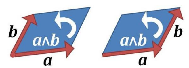
$a \wedge b$ → 벡터 a를 벡터 b로 움직이는 rotation. 두 벡터로 정의되는 평행사변형이 회전 평면이 되고, 평면의 크기가 두 벡터 사이의 bivector가 됨.

• trivector : degree 3를 갖는 multi-vector

bivector $B$에 의해 정의된 rotation $R$ (rotor)은 다음과 같이 정의함. (회전하고자 하는 각도 $\theta$)

$R=\text{exp}(-B\frac{\theta}{2})=e^{-B\frac{\theta}{2}}$

3. Bivector

Exterior product

dot product, cross product

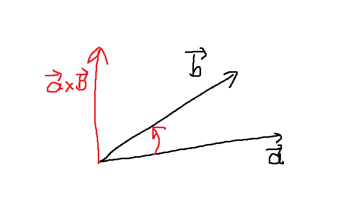
• dot product ($a\cdot b$) (내적) : 스칼라곱 → 스칼라 값을 return함. $\vec{a} \cdot \vec{b} = \vec{a} \vec{b} \ |\cos\theta|$
  • $(a_1,a_2)\cdot(b_1, b_2)=a_1b_1+a_2b_2$
• cross product($a \times b$) (외적) : $\vec{a}$와 $\vec{b}$에 모두 수직인 새로운 벡터를 return. 외적의 크기는 $\vec{a}, \vec{b}$가 이루는 평행사변형의 넓이와 같음. (오른손 법칙 적용)
  • $\vec{a}\times\vec{b}= \ \begin{vmatrix}x & y & z \\ a_1 & a_2 & a_3 \\ b_1 & b_2 & b_3\end{vmatrix}$

---

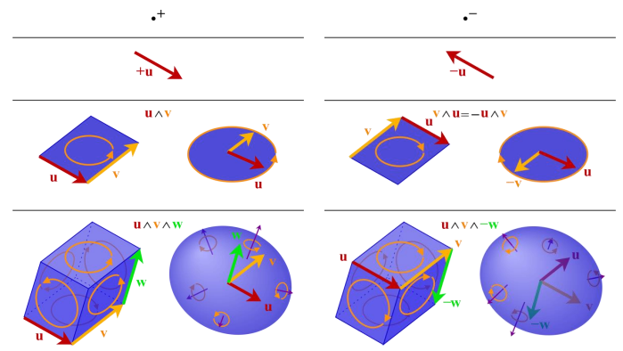
exterier product (wedge product) → $u \wedge v$ (bivector)

$u \wedge v$의 magnitude (크기)는 u, v 벡터가 이루는 평행사변형의 넓이임. → magnitude에 한해 3차원 상에서의 cross product와 동일함.

u, v의 평면과 평행한 모든 평면은 같은 bivector로 표현이 가능함.

cross product와 마찬가지로 교환법칙이 성립하지 않음. → $u\wedge v=-(v \wedge u)$

but, cross product와 달리 결합법칙은 성립함. → $(u\wedge v)\wedge w = u\wedge (v \wedge w)$

(IK에서는 대부분 2차원 선에서 해결됨.)

---

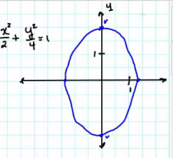
cartesian plane $\R^2$는 다음 두 개의 unit vector로 구성되어 있음.

$e_1=\begin{bmatrix}1\\ 0\end{bmatrix}, \ e_2=\begin{bmatrix}0\\ 1\end{bmatrix}$ ($e_1$은 x축, $e_2$는 y축이라고 생각)

이때 두 벡터 $v=\begin{bmatrix}a \\ b\end{bmatrix}=ae_1+be_2, \ w=\begin{bmatrix}c \\ d\end{bmatrix}=ce_1+de_2$를 가정함.

두 벡터로 만들어지는 평행사변형의 넓이는 다음과 같음.

$\text{Area}=|\det\begin{bmatrix}v & w\end{bmatrix}|=|\det\begin{bmatrix}a & c \\ b & d\end{bmatrix}|=|ad-bc|$

따라서

$v\wedge w=(ae_1+be_2)\wedge (ce_1+de_2) \\ = ace_1\wedge e_1+ade_1 \wedge e_2+bce_2\wedge e_1+bde_2\wedge e_2 \\ =(ad-bc)e_1\wedge e_2$

---

3차원 상에서는 oreinted vector space가 존재하는데, cross product와 triple product와 관련이 깊음.

$u\wedge v=(u_1v_2-u_2v_1)(e_1\wedge e_2)+(u_2v_3-u_3v_2)(e_2\wedge e_3)+(u_3v_1-u_1v_3)(e_3\wedge e_1)$ → 회전평면 3개에 각각 스칼라가 곱해져서 움직이는 형태

이때 $(e_1\wedge e_2, e_2\wedge e_3, e_3\wedge e_1)$은 각각 3차원 공간의 기저임.

$u\wedge v\wedge w=(u_1v_2w_3+u_2v_3w_1+u_3v_1w_2-u_1v_3w_2-u_2v_1w_3-u_3v_2w_1)(e_1\wedge e_2\wedge e_3)$ → 회전평면 1개에 스칼라 값이 곱해지는 형태

Quaternion

bivector는 quaternion과 관련이 깊음.

quaternion은 rotation을 표현하는 또다른 수단.

원래 rotation을 가장 쉽게 표현하는 방법은 euler rotaion을 사용하는 것. → 회전하고자 하는 벡터를 행렬에 곱해주는 방식으로 회전 표현

$R_x(\phi)=\begin{pmatrix}1&0&0\\0&\cos\phi&\sin\phi\\0&-\sin\phi&\cos\phi\end{pmatrix} \\ R_y(\theta)=\begin{pmatrix}\cos\theta&0&-\sin\theta\\0&1&0\\\sin\theta&0&\cos\theta\end{pmatrix} \\ R_z(\psi)=\begin{pmatrix}\cos\psi&\sin\psi&0\\-\sin\psi&\cos\psi&0\\0&0&1\end{pmatrix}$

하지만 이 방식에는 단점이 있기 때문에 이 방식보다는 quaternion을 사용하여 표현함. (quaternion은 $i,j,k$를 통해 표현함)

quaternion은 “회전을 더 잘 표현하고 사용하기 위한” 방법임.

• 기존 euler rotation의 한계는 “x, y, z축”을 기준으로 회전한다는 것임. → 회전에 제약이 존재 → quaternion은 임의의 벡터를 기준으로 회전할 수 있는 것이 장점.
• euler rotation보다 간단하고 효율적이며 numerically stable (수치적으로 원하는 형태를 잘 표현할 수 있다는 뜻)함.
• 단점 → 직관적이지 않고 이해하기 어려움. (머리가 부서질 수 있다..ㅠ)

---

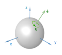
euler rotation에 따르면, 어떤 fixed point를 기준으로 하는 rigid body의 회전은 어떤 벡터 (euler axis)를 기준으로 회전하는 것으로 표현할 수 있음.

euler axis는 보통 unit vector $\vec{u}$로 표현하고, 여러 축을 기준으로 하는 회전을 하나로 합칠 수 있음.

quaternion은 이러한 회전을 4개의 숫자로 간단하게 표현하는 방법.

특정 벡터 $(x,y,z)$를 이용하여 회전을 표현할 수 있고, euler rotation ↔ quaternion은 서로 교환 가능함.

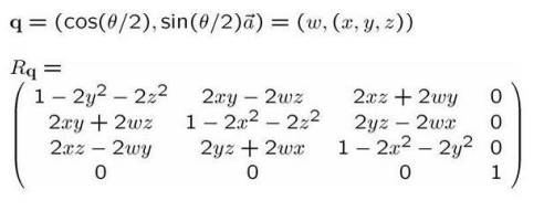
(2, 3, 4)와 같은 유클리드 벡터를 $2i+3j+4k$와 같이 표현할 수 있음. 이때 $i,j,k$는 unit vector. 또한 cartesian axis ($2e_1+3e_2+4e_3$)로 표현할 수 있음.

이때 unit vector $\vec{u}=(u_x,u_y,u_z)=u_xi+u_yj+u_zk$를 기준으로 하는 각도 $\theta$만큼의 회전은 다음과 같이 표현할 수 있음.

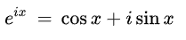
⭐$\text{q}=e^{\frac{\theta}{2}(u_xi+u_yj+u_zk)}=\cos\frac{\theta}{2}+(u_xi+u_yj+u_zk)\sin\frac{\theta}{2}$ (오일러 공식을 통한 지수 분해)

---

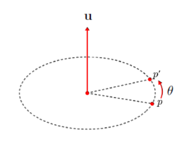
이때 $\text{q}$를 회전하고자 하는 점 $\text{p}=(p_x,p_y,p_z)$에 적용하면 다음과 같음.

$\text{p}'=\text{q}\text{p}\text{q}^{-1}$ → $\text{p}'$ : 회전을 마친 후의 새로운 position

또한 회전 행렬 $R$을 다음과 같이 표현하여 점 $\text{p}$에 곱하면 회전한 점 $\text{p}'$를 구할 수 있음. → $\text{p}'=R\text{p}$

$R=\begin{bmatrix}1-2s(q_j^2+q_k^2)&2s(q_iq_j-q_kq_r)&2s(q_iq_k+q_jq_r)\\2s(q_iq_j+q_kq_r)&1-2s(q_i^2+q_k^2)&2s(q_jq_k-q_iq_r)\\2s(q_iq_k-q_jq_r)&2s(q_jq_k+q_iq_r)&1-2s(q_i^2+q_j^2)\end{bmatrix}$

Rotation vector and rotor

geometric algebra에서는 회전을 bivector로 표현할 수 있음.

$\Omega$를 bivector의 회전 평면, $\theta$를 회전 각도라고 한다면, rotation bivector는 $\Omega\theta$임.

$e^{\frac{\Omega\theta}{2}}=\cos(\frac{\theta}{2})+\Omega\sin(\frac{\theta}{2})$ → 위에 있는 식과 비슷 (⭐)

이를 적용하여 $\text{v}$를 $\text{v}'$로 보낼 수 있음.

$\text{v}'=e^{-\frac{\Omega\theta}{2}}\text{v}e^{\frac{\Omega\theta}{2}}$

이때 $e^{-\frac{\Omega\theta}{2}}$를 rotor라고 함.

---

Reference

[1] Inverse Kinematics: ‘Inverse Kinematics: a review of existing techniques and introduction of a new fast iterative
solver, 2009’

[2] Cartesian: https://en.wikipedia.org/wiki/Cartesian_coordinate_system

[3] A. Balestrino, G. De Maria, and L. Sciavicco. Robust control of robotic manipulators. In Proceedings
of the 9th IFAC World Congress, volume 5, pages 2435–2440, 1984.

[4] W. A. Wolovich and H. Elliott. A computational technique for inverse kinematics. The 23rd IEEE
Conference on Decision and Control, 23:1359–1363, December 1984.

[5] J. Baillieul. Kinematic programming alternatives for redundant manipulators. In Proceedings of
the IEEE International Conference on Robotics and Automation, volume 2, pages 722–728, March
1985.

[6] C. W. Wampler. Manipulator inverse kinematic solutions based on vector formulations and damped
least-squares methods. Proceeding of the IEEE Transactions on Systems, Man and Cybernetics,
16(1):93–101, 1986.

[7] Y. Nakamura and H. Hanafusa. Inverse kinematic solutions with singularity robustness for robot
manipulator control. Trans. ASME, Journal of Dynamic Systems, Measurement, and Control,
108(3):163–171, September 1986.

[8] Samuel R. Buss and Jin-Su Kim. Selectively damped least squares for inverse kinematics. Journal
of Graphics Tools, 10(3):37–49, 2005.

[9] BFGS: ‘Practical methods of optimization, 2013’