본 포스트는 < Understanding Deep Learning : Application in Rare Event Prediction >의 저자 Chitta Ranjan의 글을 바탕으로 작성되었습니다.

Background

Extreme Rare Event

제조업에서의 기계 고장 탐지와 같은 Rare Event Problem에서는, positively labeled data보다 negatively labeled data가 훨씬 많은 불균형한 데이터셋을 다루게 됩니다.

	Typical rare-event	Extreme rare-event
positively labeled data	5~10%	less than 1%

그 중 positively labeled data가 전체 데이터의 1%가 채 되지 않을 때 해당 문제는 'Extreme rare-event problem'으로 정의됩니다.

이렇게 positively labeled data 비율이 극히 낮을 경우에는, 딥러닝 기법을 적용하여 문제를 해결하기가 어렵습니다. 데이터셋의 불균형은 학습의 불균형으로 이어지기 때문입니다.

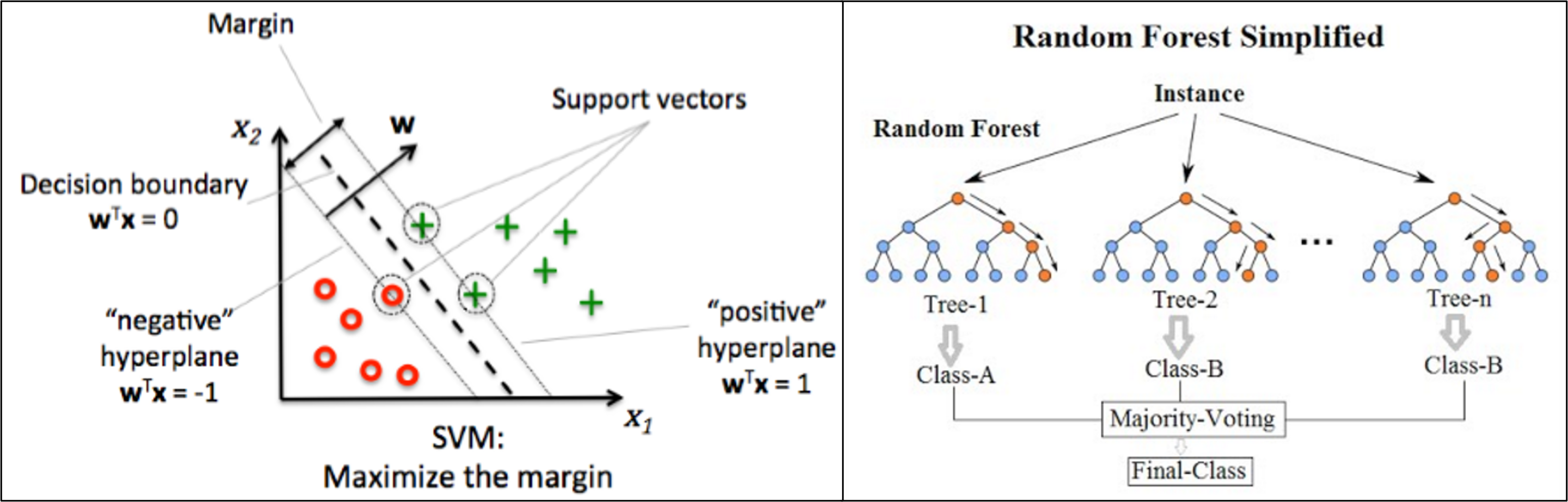
물론, 딥러닝 기법을 적용하지 않고 Undersampling을 거쳐 SVM(Support Vector Machine)이나 RandomForest 등의 머신러닝 기법으로 문제를 해결할 수는 있습니다.

하지만 아래와 같은 문제가 있습니다.

• Undersampling으로 인해 정보 활용도가 낮아짐
  • Extreme rare-event problem에서는 Undersampling으로 negatively labeled data의 비율을 조정할 경우, 남은 데이터(전체의 98~99%)에 포함된 정보는 활용할 수 없게 됩니다.
• Accuracy의 한계

따라서, 데이터셋이 충분한 경우에는 딥러닝 기법을 적용하여 Extreme rare-event problem을 해결하는 편이 바람직합니다. (데이터셋이 내포하는 정보를 최대한 활용하면서, 구조를 바꿔가면서 모델 성능을 높일 수 있기에 유연합니다.)

본 포스팅에서는 AutoEncoder에 기반한 Rare-Event classifier의 구조를 먼저 살펴보고, Time-Series data에 적용할 LSTM-AutoEncoder에 대해 소개하겠습니다.

[참고] Anomaly Detection과 Binary Classifier

• Anomaly Detection에서는 모델이 정상 과정(normal process)의 패턴을 학습하고, 새로 들어온 데이터가 해당 패턴을 따른다면 정상 데이터, 벗어난다면 anomaly로 분류합니다.
• 이는 rare-event에 대한 binary classification과 유사한 방법론이기에, 본 포스팅에서는 anomaly를 rare-event의 한 범주로 생각하셔도 무방합니다.

AutoEncoder

AutoEncoder 구조

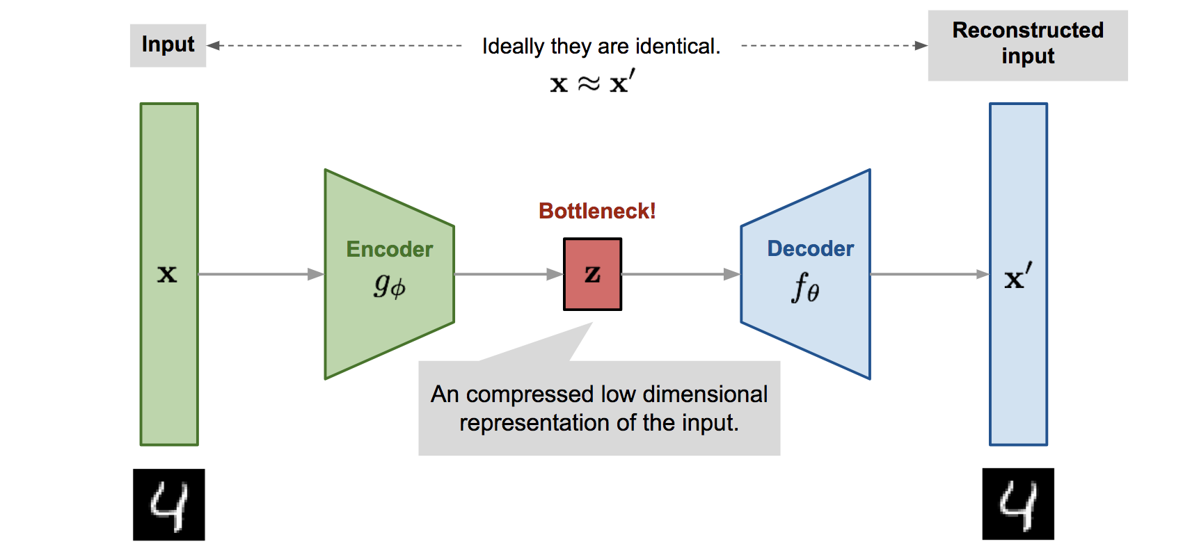
• Self-supervised Learning
• Input(x) → Encoder → Decoder → Output(x')
• AutoEncoder의 Encoder와 Decoder는 대칭 구조입니다.
• Encoder에서는 주어진 Input을 차원 축소를 통해 latent vector로 변환(representation)하는데, 차후 Input을 재구성해야 하기에 정보를 잘 압축하는 것이 중요합니다.
• Decoder는 일종의 Generator인데, Latent Vector를 이용해 Input을 재구성(reconstruction)합니다.
• 이렇게 재구성된 Output(x')과 Input의 차이를 계산하면 reconstruction error가 얻어집니다.
  • AutoEncoder의 학습(parameter update)은 이 reconstruction error를 줄이는 방향으로 이루어집니다.

AutoEncoder Rare-Event Classifier

Classification은 아래와 같이 진행됩니다.

1) 전체 데이터를 positively labeled data(rare event, 이하 'anomaly')와 negatively labeled data(normal process, 이하 'normal data') 두 종류로 분류

2) AutoEncoder 학습 (※ normal data만 이용)

3) 2)의 결과로 AutoEncoder는 normal data의 주요 feature를 파악하게 되므로, 잘 학습되었다면 normal process에서 파생된 새로운 데이터(즉, 새로운 normal data)에 대한 reconstruction을 훌륭하게 수행

4) 하지만, 새로운 데이터로 anomaly가 들어온다면 reconstruction이 제대로 수행되지 않을 것 (AutoEncoder는 학습 과정에서 anomaly를 다루지 않았음)

5) 따라서, 일정 수준 이상(cutoff)의 high reconstruction error를 발생시키는 데이터는 anomaly로 라벨링

위 과정을 파이썬으로 구현한 예시는 이곳에서 확인하실 수 있습니다.
(Dataset : Binary labeled data from a pulp-and-paper mill for sheet breaks)

LSTM AutoEncoder

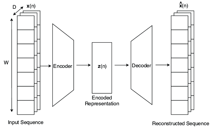
위에서는 Simple Dense Layer AutoEncoder로 Classifier를 구성했으나, 해당 Classifier는 sequence data나 time-series data의 시간적(temporal) 특성을 파악하지 못하는 문제가 있습니다.

이때 LSTM AutoEncoder에 기반한 Classifier를 구성함으로써 위 문제를 해결할 수 있습니다.
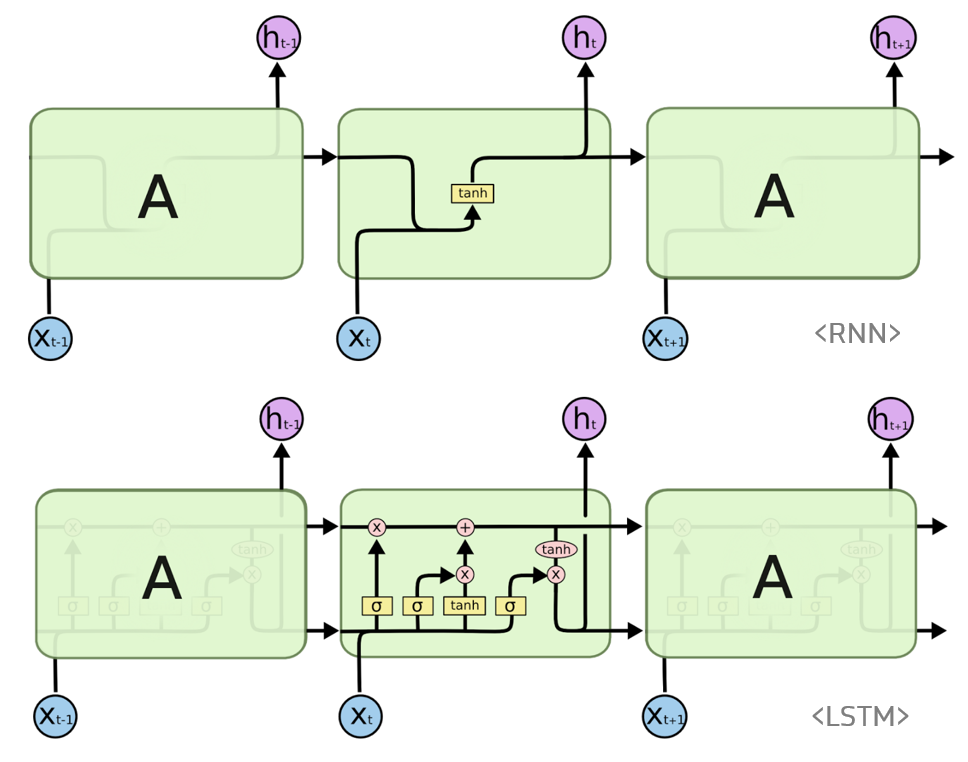
LSTM(Long Short-Term Memory Network)은 RNN(Recurrent Neural Network)의 일종으로, 과거 event의 long-term effects와 short-term effects를 모두 파악할 수 있습니다.

LSTM AutoEncoder의 구조는 아래와 같습니다.

Code Review

출처 : https://github.com/cran2367/lstm_autoencoder_classifier/blob/master/lstm_autoencoder_classifier.ipynb

위 Github에서 전체 코드를 확인하실 수 있으며, 본 포스트에는 LSTM AutoEncoder Building 및 Training을 위한 주요 코드만을 첨부했습니다.

먼저, 필요한 라이브러리와 패키지를 불러옵니다.

%matplotlib inline
import matplotlib.pyplot as plt
import seaborn as sns

import pandas as pd
import numpy as np
from pylab import rcParams

import tensorflow as tf
from keras import optimizers, Sequential
from keras.models import Model
from keras.utils.vis_utils import plot_model
from keras.layers import Dense, LSTM, RepeatVector, TimeDistributed
from keras.callbacks import ModelCheckpoint, TensorBoard

from sklearn.preprocessing import StandardScaler
from sklearn.model_selection import train_test_split
from sklearn.metrics import confusion_matrix, precision_recall_curve
from sklearn.metrics import recall_score, classification_report, auc, roc_curve
from sklearn.metrics import precision_recall_fscore_support, f1_score

from numpy.random import seed
seed(7)
tf.random.set_seed(11)

from sklearn.model_selection import train_test_split

SEED = 123   # used to help randomly select the data points
DATA_SPLIT_PCT = 0.2

rcParams['figure.figsize'] = 8, 6
LABELS = ["Normal","Break"]

LSTM Model의 Input은 [data_size, time_steps, features]로 구성된 3차원 array여야 하므로, 이에 맞추어 데이터셋을 가공합니다.

1) 데이터 불러오기

df = pd.read_csv('processminer-rare-event-mts - data.csv') 
df.head(n = 5)   # time column, 1개의 binary response variable(y), 그리고 61개의 predictor(x1~x61) 

2-1) 데이터 Shifting

• 이번 Rare-Event Problem의 목적은 sheet-break을 미리 예측하는 것입니다.
• df.y=df.y.shift(-2)로 각 label로 이전 두 행의 label로 채움으로써 최대 4분 먼저 sheet-break을 predict할 수 있습니다.
• 이때 본 코드에서는 단순 shifting에 그치지 않고, n번째 label의 shifting 및 n번째 행 제거를 수행하는 규칙을 따릅니다(아래 주석 참고).

sign = lambda x: (1, -1)[x < 0]

def curve_shift(df, shift_by):
    '''
    This function will shift the binary labels in a dataframe.
    The curve shift will be with respect to the 1s. 
    For example, if shift is -2, the following process
    will happen: if row n is labeled as 1, then
    - Make row (n+shift_by):(n+shift_by-1) = 1.
    - Remove row n.
    i.e. the labels will be shifted up to 2 rows up.
    
    Inputs:
    df       A pandas dataframe with a binary labeled column. 
             This labeled column should be named as 'y'.
    shift_by An integer denoting the number of rows to shift.
    
    Output
    df       A dataframe with the binary labels shifted by shift.
    '''

    vector = df['y'].copy()
    for s in range(abs(shift_by)):
        tmp = vector.shift(sign(shift_by))
        tmp = tmp.fillna(0)
        vector += tmp
    labelcol = 'y'
    # Add vector to the df
    df.insert(loc=0, column=labelcol+'tmp', value=vector)
    # Remove the rows with labelcol == 1.
    df = df.drop(df[df[labelcol] == 1].index)
    # Drop labelcol and rename the tmp col as labelcol
    df = df.drop(labelcol, axis=1)
    df = df.rename(columns={labelcol+'tmp': labelcol})
    # Make the labelcol binary
    df.loc[df[labelcol] > 0, labelcol] = 1

    return df

2-2) Shifting 결과 확인 (Before vs After)

• 259(n)번째 행의 label이 1이므로, 먼저 258(n-1)번째, 257(n-2)번째 행의 label을 1로 채웁니다. 이후 259번째 행은 제거합니다(sheet-break이 발생한 이후의 prediction은 의미가 없기 때문입니다).

'''
Shift the data by 2 units, equal to 4 minutes.

Test: Testing whether the shift happened correctly.
'''
print('Before shifting')   # Positive labeled rows before shifting.
one_indexes = df.index[df['y'] == 1]
display(df.iloc[(one_indexes[0]-3):(one_indexes[0]+2), 0:5].head(n=5))

# Shift the response column y by 2 rows to do a 4-min ahead prediction.
df = curve_shift(df, shift_by = -2)

print('After shifting')   # Validating if the shift happened correctly.
display(df.iloc[(one_indexes[0]-4):(one_indexes[0]+1), 0:5].head(n=5))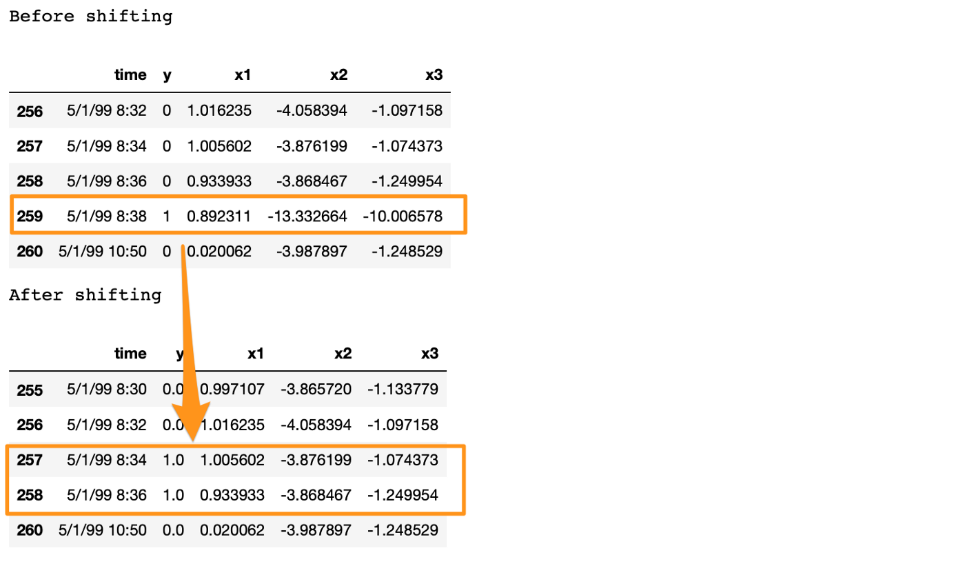

3) 데이터 Cleaning

# Remove time column, and the categorical columns
df = df.drop(['time', 'x28', 'x61'], axis=1)

4) 3차원 array 생성 (LSTM Model의 Input)

• 앞서 기술했듯이, LSTM Model의 Input은 [data_size(이하 'samples'), time_steps(이하 'lookback'), features]로 구성된 3차원 array여야 합니다.
• samples는 데이터 개수, lookback은 특정 데이터가 처리(process)할 과거 데이터 개수, features는 Input의 feature 수를 말합니다.

input_X = df.loc[:, df.columns != 'y'].values   # converts the df to a numpy array
input_y = df['y'].values

n_features = input_X.shape[1]   # number of features

위 코드에서 input_X는 [samples, features]로 구성된 2차원 array이므로, lookback을 포함하는 3차원 array로 변환되어야 합니다.
변환을 위해 필요한 함수가 바로 아래의 temporalize입니다.

• temporalize의 input은 2차원 array X(samples*n_features), X에 대응하는 1차원 array y(samples), 그리고 window size(몇 개의 과거 데이터를 처리할지)인 lookback으로 구성됩니다.
• temporalize의 output은 3차원 array output_X((samples-lookback-1)lookbackn_features), 그리고 output_X에 대응하는 1차원 array output_y(samples-lookback-1)로 구성됩니다.

def temporalize(X, y, lookback):
    output_X = []
    output_y = []
    for i in range(len(X)-lookback-1):
        t = []
        for j in range(1,lookback+1):
            # Gather past records upto the lookback period
            t.append(X[[(i+j+1)], :])
        output_X.append(t)
        output_y.append(y[i+lookback+1])
    return output_X, output_y

temporalize 함수가 잘 정의되었는지 검증하기 위해, lookback=5로 설정한 후 첫 번째 sheet-break 데이터에 대한 결과를 확인해보겠습니다.

'''
Test: The 3D tensors (arrays) for LSTM are forming correctly.
'''
print('First instance of y = 1 in the original data')
display(df.iloc[(np.where(np.array(input_y) == 1)[0][0]-5):(np.where(np.array(input_y) == 1)[0][0]+1), ])

lookback = 5   # Equivalent to 10 min of past data.
# Temporalize the data
X, y = temporalize(X = input_X, y = input_y, lookback = lookback)

print('For the same instance of y = 1, we are keeping past 5 samples in the 3D predictor array, X.')
display(pd.DataFrame(np.concatenate(X[np.where(np.array(y) == 1)[0][0]], axis=0 )))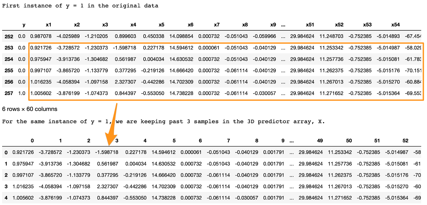 

두 테이블의 결과가 동일한 것으로 보아, temporalize 함수는 잘 정의되었습니다.
5) 데이터 Split : Train/Validation/Test

X_train, X_test, y_train, y_test = train_test_split(np.array(X), np.array(y), test_size=DATA_SPLIT_PCT, random_state=SEED)
X_train, X_valid, y_train, y_valid = train_test_split(X_train, y_train, test_size=DATA_SPLIT_PCT, random_state=SEED)

X_train.shape   # (11691, 5, 1, 59)

LSTM AutoEncoder Training에서는 negatively labeled data(즉, y가 0인 data)만을 사용하므로, Train과 Validation 데이터를 한 번 더 분리해줍니다.

X_train_y0 = X_train[y_train==0]
X_train_y1 = X_train[y_train==1]

X_valid_y0 = X_valid[y_valid==0]
X_valid_y1 = X_valid[y_valid==1]

X_train_y0.shape   # (11536, 5, 1, 59)

• 마지막으로, Input을 모두 3차원으로 reshape합니다.

X_train = X_train.reshape(X_train.shape[0], lookback, n_features)
X_train_y0 = X_train_y0.reshape(X_train_y0.shape[0], lookback, n_features)
X_train_y1 = X_train_y1.reshape(X_train_y1.shape[0], lookback, n_features)

X_test = X_test.reshape(X_test.shape[0], lookback, n_features)

X_valid = X_valid.reshape(X_valid.shape[0], lookback, n_features)
X_valid_y0 = X_valid_y0.reshape(X_valid_y0.shape[0], lookback, n_features)
X_valid_y1 = X_valid_y1.reshape(X_valid_y1.shape[0], lookback, n_features)

6) 데이터 Standardizing

• 일반적으로 AutoEncoder의 Input으로는 standardized data를 사용합니다.
• 이때 Standardization 자체는 가공된 3차원 array가 아닌 원본 데이터(2차원)에 대해 수행되어야 하므로, 데이터 스케일링을 위해 추가로 함수를 정의해야 합니다. (flatten, scale)
  • flatten : temporalize의 inverse function (3차원 array를 original 2차원 array로 recreate)
  • scale : LSTM AutoEncoder의 Input인 3차원 array에 대한 스케일링 수행

def flatten(X):
    '''
    Flatten a 3D array.
    
    Input
    X            A 3D array for lstm, where the array is sample x timesteps x features.
    
    Output
    flattened_X  A 2D array, sample x features.
    '''
    flattened_X = np.empty((X.shape[0], X.shape[2]))  # sample x features array.
    for i in range(X.shape[0]):
        flattened_X[i] = X[i, (X.shape[1]-1), :]
    return(flattened_X)


def scale(X, scaler):
    '''
    Scale 3D array.

    Inputs
    X            A 3D array for lstm, where the array is sample x timesteps x features.
    scaler       A scaler object, e.g., sklearn.preprocessing.StandardScaler, sklearn.preprocessing.normalize
    
    Output
    X            Scaled 3D array.
    '''
    for i in range(X.shape[0]):
        X[i, :, :] = scaler.transform(X[i, :, :])
        
    return X

• X_train_y0를 이용해 Standardization 객체를 fit합니다.

# Initialize a scaler using the training data
scaler = StandardScaler().fit(flatten(X_train_y0))

• fit된 scaler를 이용해 모든 Input에 대한 스케일링을 수행합니다.

X_train_y0_scaled = scale(X_train_y0, scaler)
X_train_y1_scaled = scale(X_train_y1, scaler)
X_train_scaled = scale(X_train, scaler)

X_valid_scaled = scale(X_valid, scaler)
X_valid_y0_scaled = scale(X_valid_y0, scaler)

X_test_scaled = scale(X_test, scaler)

7) LSTM AutoEncoder Training

• 본격적으로 학습을 진행합니다. 아래는 초기 설정입니다.

timesteps =  X_train_y0_scaled.shape[1]   # equal to the lookback
n_features =  X_train_y0_scaled.shape[2]   # 59

epochs = 200
batch = 64
lr = 0.0001

• Simple LSTM AutoEncoder를 구축합니다.

lstm_autoencoder = Sequential()

# Encoder
lstm_autoencoder.add(LSTM(32, activation='relu', input_shape=(timesteps, n_features), return_sequences=True))
lstm_autoencoder.add(LSTM(16, activation='relu', return_sequences=False))
lstm_autoencoder.add(RepeatVector(timesteps))

# Decoder
lstm_autoencoder.add(LSTM(16, activation='relu', return_sequences=True))
lstm_autoencoder.add(LSTM(32, activation='relu', return_sequences=True))
lstm_autoencoder.add(TimeDistributed(Dense(n_features)))

lstm_autoencoder.summary()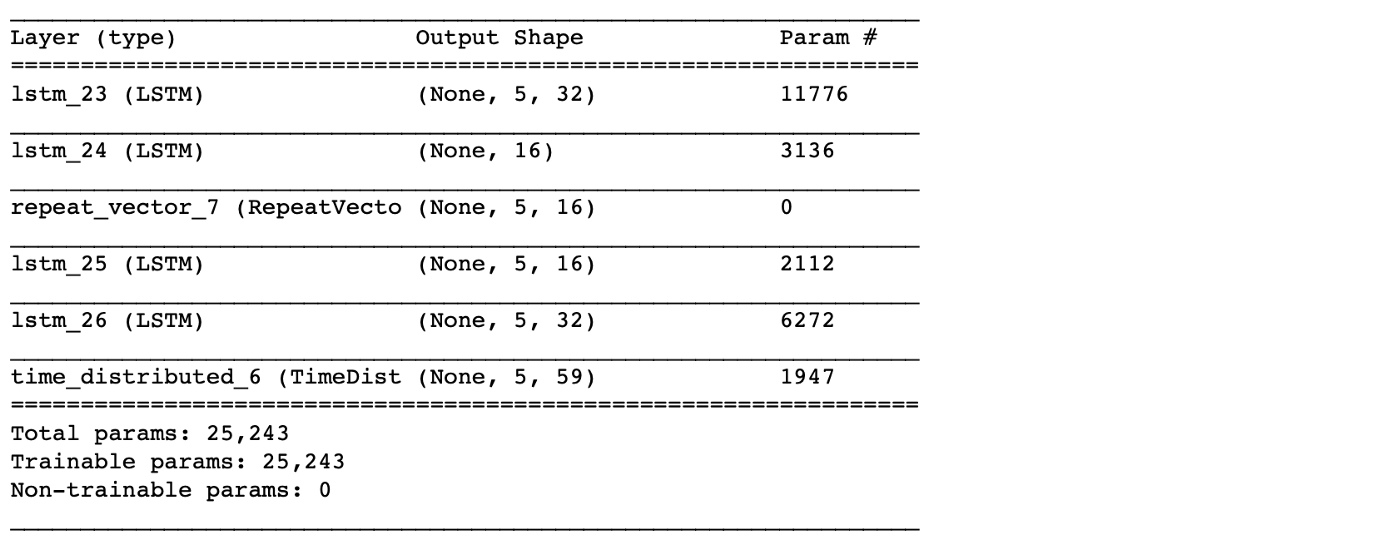

adam = tf.keras.optimizers.Adam(lr)   # Adam Optimizer
lstm_autoencoder.compile(loss='mse', optimizer=adam)   # MSE loss

cp = ModelCheckpoint(filepath="lstm_autoencoder_classifier.h5",
                               save_best_only=True,
                               verbose=0)

tb = TensorBoard(log_dir='./logs',
                histogram_freq=0,
                write_graph=True,
                write_images=True)

lstm_autoencoder_history = lstm_autoencoder.fit(X_train_y0_scaled, X_train_y0_scaled, 
                                                epochs=epochs, 
                                                batch_size=batch, 
                                                validation_data=(X_valid_y0_scaled, X_valid_y0_scaled),
                                                verbose=2).history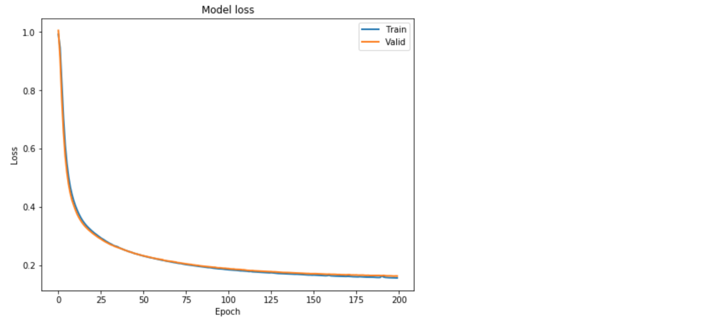

[참고]
LSTM AutoEncoder Layer에 대한 단계별 이해

Further Improvement : ConvLSTM

앞서 LSTM AutoEncoder 기반으로 Rare-Event Classifier를 구축하는 과정을 살펴보았는데, 이외에도 아래처럼 다양한 모델을 융합함으로써 Anomaly Detection을 수행할 수 있습니다.

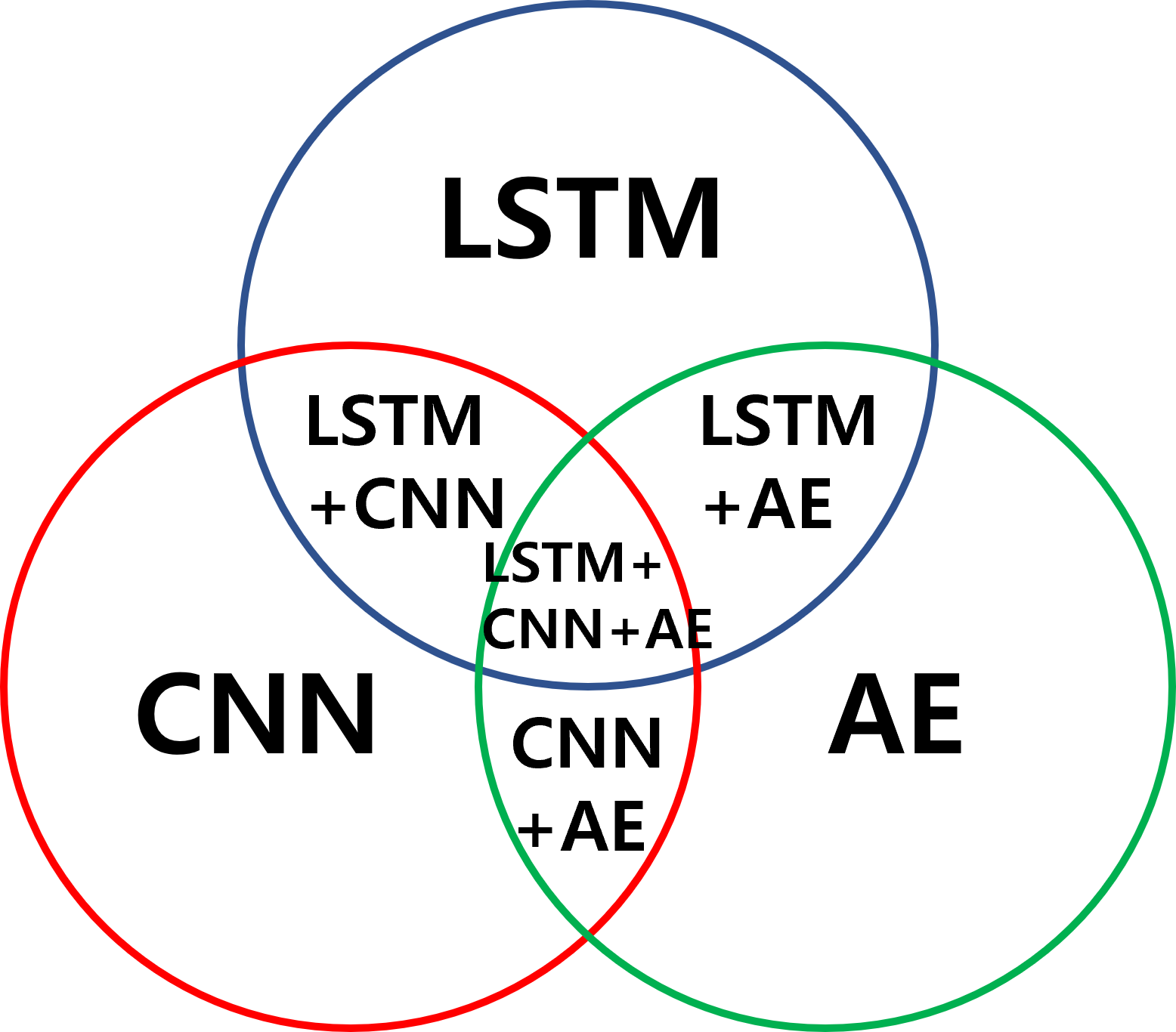
이중 LSTM과 CNN의 융합 모델인 Convolutional LSTM - 시계열 자료를 활용한 해수면 온도 예측 딥러닝 모델에 대해 추가로 소개합니다.
아래 내용은 DSBA Seminar 자료 및 이곳을 참고하여 작성되었습니다.

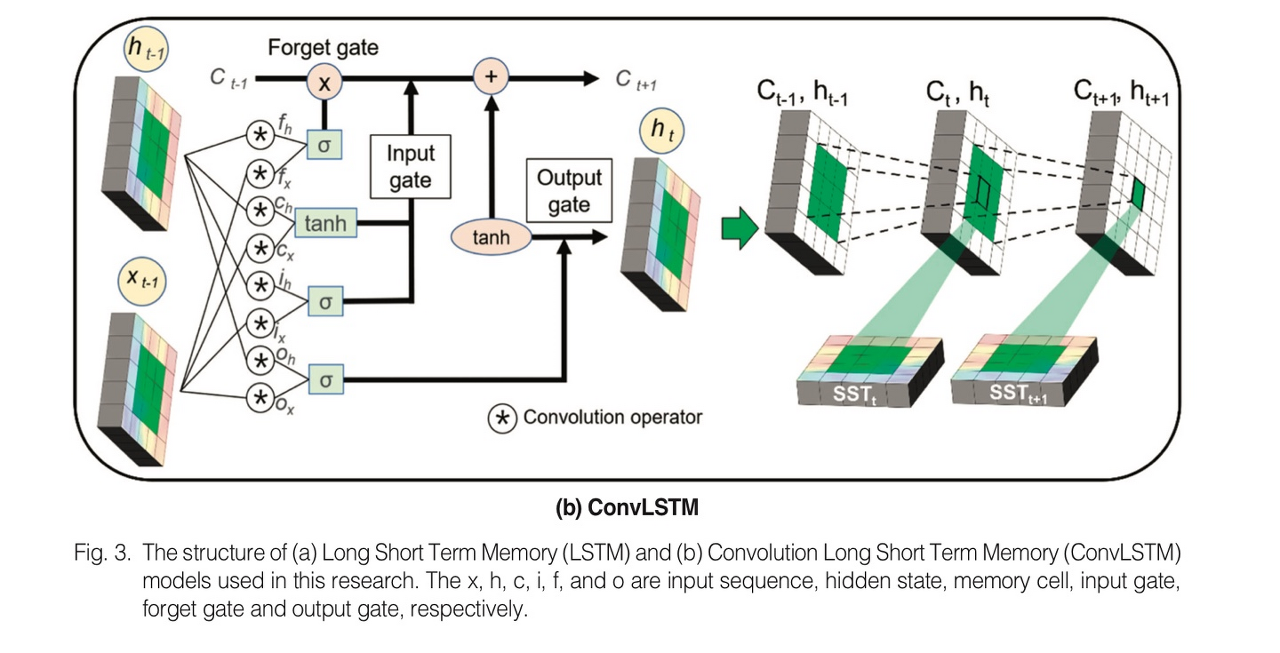
ConvLSTM의 기법은 다음과 같습니다.

• CNN은 Spatial pattern mining에 사용되고, LSTM은 Temporal pattern recognition에 사용됩니다.
• 따라서, CNN과 LSTM을 융합하면 공간적 정보와 시간적 정보를 모두 파악할 수 있습니다.
• ConvLSTM은 입력, 출력, 상태 레이어가 3차원 벡터로 연산(기존 LSTM 모델에서는 1차원)되며 일반 행렬곱 대신 합성곱(Convolutional Operation)으로 이루어져 시간적, 공간적 특성을 동시에 학습할 수 있다는 장점이 있습니다. 또 기존 LSTM 모델보다 우수한 성능을 갖습니다.
  
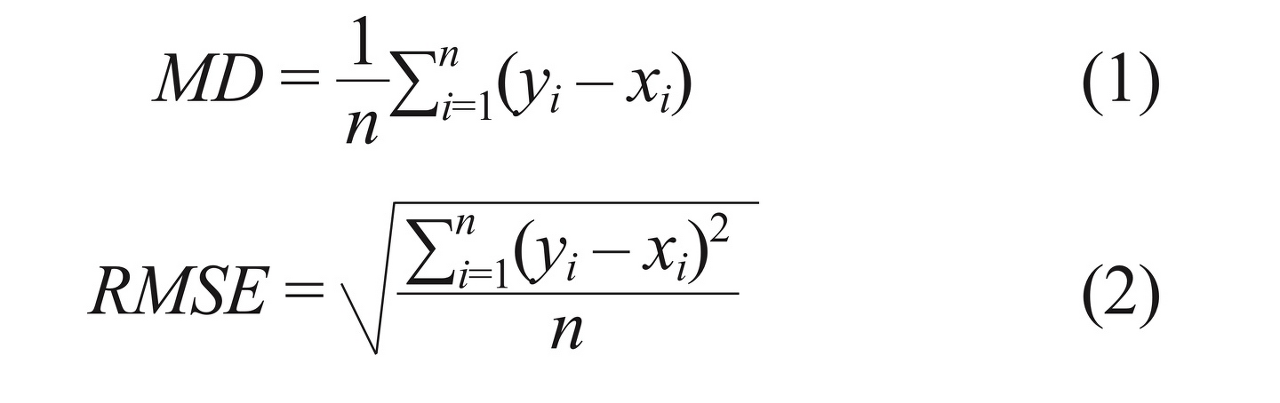
• Accuracy 지표로는 평균오차(Mean Difference: MD)와 RMSE(Root Mean Sqaure Error)가 사용되었습니다.
  • MD는 과추정, 저추정과 같은 공간적 오차의 패턴 분석에 용이합니다.
  • RMSE는 공간적 오차의 절대적 분포를 비교하는데 용이합니다.
    

연구 결과에 대한 요약은 다음과 같습니다.

• 예측 오차 변화 분석

  • 예측 기간이 길어짐에 따라 LSTM 모델의 RMSE가 ConvLSTM과 비교하여 빠르게 증가하고, 전체 기간보다는 여름철의 예측 오차가 더 빠르게 증가합니다.
  • 오차 증가폭은 LSTM이 ConvLSTM보다 큰데, 합성곱을 활용한 연산의 성능 향상에서 그 원인을 찾을 수 있습니다.

• 일일 해수면 온도 예측 결과 정확도 분석

  • 전 계절을 통틀어서나, 개별적으로나 ConvLSTM 모델의 예측 정확도가 LSTM 모델과 비교하여 높았습니다.
  • LSTM 모델은 공간 분포에 대해 높은 노이즈를 보이는데, 이를 해결하기 위해 픽셀의 공간적 특성을 반영하는 CNN을 적용한 FC-LSTM이나 ConvLSTM을 활용할 수 있습니다.

• 예측 기간별 공간적 오차 분석

  • LSTM, ConvLSTM 두 모델 모두 예측 일수가 증가할수록 예측 오차가 증가했으며, MD 측면에서 LSTM은 불연속적인 오차 패턴을, ConvLSTM은 연속적인 양의 오차를 보였습니다.

• 고수온 영역 탐지 활용 결과

  • 고수온이 발생한 2017-8-17일 레퍼런스 자료로부터 ConvLSTM의 예측 결과가 LSTM보다 더 유사한 공간적 분포를 가졌습니다.
  • 이상치 측면에서도 LSTM 모델은 예측 기간이 2일 이상일 때 급격한 성능 저하가 나타나는 반면, ConvLSTM 모델은 예측 기간이 5일을 넘어서는 순간부터 예측 오차가 서서히 증가하는 경향이 있습니다.

Reference

• Extreme Rare Event Classification using Autoencoders in Keras
• LSTM Autoencoder for Extreme Rare Event Classification in Keras
• Step-by-step understanding LSTM Autoencoder layers
• [Paper Review] Anomaly Detection in Time Series
  (강의 영상 : https://www.youtube.com/watch?v=lqt3OEI3N1A)