CNN for univariate/multivariate/multi-step/multivariate multi-step TSF
CNN은 이미지 데이터 뿐만 아니라 시계열 예측(Time Seires Forecasting)에도 적용될 수 있습니다. 다양한 유형의 시계열 예측 문제에 적용가능한 CNN의 종류는 다양하고 이번 주차에서는 CNN for Univariate/Multivariate/Multi-step/Multivariate Multi-step Time Series Forcasting에 대한 내용을 살펴보도록 하겠습니다.
1. Univariate CNN Models
Univariate Time Series (일변량 시계열) 는 시간적 순서가 있는 단일 관측치 시리즈로 구성되어 있습니다. 과거의 관측치들로부터 sequence의 다음 값을 예측하기 위해 CNN을 사용하게 됩니다.
1.1 Data Preparation
# univariate data preparation
from numpy import array

# split a univariate sequence into samples  -> 주어진 일변량 시계열을 여러 개의 샘플로 분할(input/output)
def split_sequence(sequence, n_steps):
    X, y = list(), list()
    for i in range(len(sequence)):
        # find the end of this pattern
        end_ix = i + n_steps
        # check if we are beyond the sequence
        if end_ix > len(sequence)-1:
            break
        # gather input and output parts of the pattern
        seq_x, seq_y = sequence[i:end_ix], sequence[end_ix]
        X.append(seq_x)
        y.append(seq_y)
    return array(X), array(y)

# define input sequence (univariate)
raw_seq = [10, 20, 30, 40, 50, 60, 70, 80, 90]

# choose a number of time steps
n_steps = 3

# split into samples
X, y = split_sequence(raw_seq, n_steps)

# summarize the data
for i in range(len(X)):
    print(X[i], y[i])
[10 20 30] 40
[20 30 40] 50
[30 40 50] 60
[40 50 60] 70
[50 60 70] 80
[60 70 80] 90
CNN 모델을 돌리기 전에 sequence를 여러 개의 input, output sample로 나누어야 하며, 예제에서는 3개의 time steps가 input으로 사용되고 one-step predictiond으로 1개의 time step이 output으로 사용됩니다. split_sequence() 함수의 경우 일변량 시계열을 여러 개의 샘플로 나누어주는 과정을 구현하고 있으며 위의 코드를 수행하면 일변량 시리즈가 6개의 샘플로 분할되며, 각 샘플에는 3개의 time step과 1개의 output time step으로 구성되어 있습니다.
1.2 CNN Model
- 1D CNN (Conv1D)
일반적인 CNN은 보통 이미지 분류에 사용되는 2D를 통칭하며, input data 형태에 따라 1D, 2D, 3D 형태의 CNN 모델이 사용됩니다. 1D CNN은 1D sequence에서 작동하는 convolutional hidden layer를 가진 CNN 모델입니다.
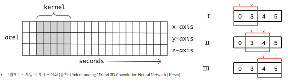
그림 5-1은 1D CNN에서 커널의 움직임을 1차적으로 시각화 한 그림입니다. 시간의 흐름에 따라 커널이 오른쪽으로 이동합니다. 시계열 데이터(Time-Series Data)를 다룰 때에는 1D CNN이 적합합니다. 1D CNN을 활용하게 되면 변수 간의 지엽적인 특징을 추출할 수 있게 됩니다.
# 일변량 시계열 예측을 위한 1D CNN 모델

from keras.models import Sequential
from keras.layers import Dense
from keras.layers import Flatten
from keras.layers.convolutional import Conv1D
from keras.layers.convolutional import MaxPooling1D

# reshape from [samples, timesteps] into [samples, timesteps, features]
n_features = 1
X = X.reshape((X.shape[0], X.shape[1], n_features)) ## (6, 3, 1)

# define model
model = Sequential()
model.add(Conv1D(filters=64, kernel_size=2, activation='relu', input_shape=(n_steps, n_features)))
model.add(MaxPooling1D(pool_size=2))
model.add(Flatten())
model.add(Dense(50, activation='relu'))
model.add(Dense(1))
model.compile(optimizer='adam', loss='mse')

# fit model
model.fit(X, y, epochs=1000, verbose=0)

# demonstrate prediction
x_input = array([70, 80, 90])
x_input = x_input.reshape((1, n_steps, n_features)) # [samples, timesteps, features]
yhat = model.predict(x_input, verbose=0)
print(yhat)
[[101.505165]]
일변량 시계열이기 때문에 feature의 개수는 1개로 설정하게 되고, CNN 모델의 input shape을 [samples, time steps, features] 3차원에 맞춰서 변환해주어야 합니다.
새로운 관측치 [70,80,90]에 대한 예측값은 101.5임을 알 수 있습니다.
2. Multivariate CNN Models
Multivariate Time Series (다변량 시계열) 는 각 time step에 대해 2개 이상의 관측치가 존재하는 데이터를 의미하며, 다변량 시계열의 2가지 주요 모델은 다음과 같습니다.
1) Multiple Input Series (다중 입력 시리즈)
2) Multiple Parallel Series (다중 병렬 시리즈)
2.1 Multiple Input Series
Multiple Input Series는 2개 이상의 parallel input time series (병렬 인풋 시계열)와 input time series에 종속된 output series를 가집니다. input time series는 동일한 time step에서의 관측치를 가지고 있기 때문에 parallel 합니다. 이를 output series가 2개의 input series의 단순 합으로 표현되는 간단한 예를 통해 확인해보겠습니다.
2.1.1 Data Preparation
# multivariate data preparation
from numpy import array
from numpy import hstack
# define input sequence
in_seq1 = array([10, 20, 30, 40, 50, 60, 70, 80, 90])
in_seq2 = array([15, 25, 35, 45, 55, 65, 75, 85, 95])
out_seq = array([in_seq1[i]+in_seq2[i] for i in range(len(in_seq1))])
# convert to [rows, columns] structure
in_seq1 = in_seq1.reshape((len(in_seq1), 1))
in_seq2 = in_seq2.reshape((len(in_seq2), 1))
out_seq = out_seq.reshape((len(out_seq), 1))
# horizontally stack columns
dataset = hstack((in_seq1, in_seq2, out_seq))
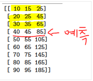
print(dataset)[[ 10 15 25][ 20 25 45]
[ 30 35 65][ 40 45 85]
[ 50 55 105][ 60 65 125]
[ 70 75 145][ 80 85 165]
[ 90 95 185]]
input 시계열은 in_seq1과 in_seq2로 정의되며, output 시계열은 2개의 input series의 합인 out_seq으로 정의됩니다. 이를 matrix 형태로 변환해주면 위와 같이 각 time step마다 2개의 input series, 1개의 output series가 있는 데이터셋이 반환됩니다. CNN은 이러한 parallel time series를 channel로 지원하고 있으며, 만약 time step을 3으로 정의하면, 첫 번째 샘플은 다음과 같습니다.
[input]
10, 15
20, 25
30, 35
[output]
65
즉, 각 parallel series의 처음 3 time step이 모델의 입력으로 제공되며, 모델은 이를 3번째 time step의 output series 값(65)과 연결합니다. 이를 통해 모델을 학습시키기 위해 시계열을 input/output sample로 변환할 때, 이전 time step에서 input series 값이 없는 output series의 값을 일부 버려야함을 알 수 있습니다. 결과적으로, input time steps size 선정은 학습 데이터를 얼마나 사용할것인지에 중요한 영향을 미침을 알 수 있습니다.
# split a multivariate sequence into samples
def split_sequences(sequences, n_steps):
    X, y = list(), list()
    for i in range(len(sequences)):
        # find the end of this pattern
        end_ix = i + n_steps
        # check if we are beyond the dataset
        if end_ix > len(sequences):
            break
        # gather input and output parts of the pattern
        seq_x, seq_y = sequences[i:end_ix, :-1], sequences[end_ix-1, -1]
        X.append(seq_x)
        y.append(seq_y)
    return array(X), array(y)

# choose a number of time steps
n_steps = 3

#convert into input/output
X, y = split_sequences(dataset, n_steps)
print(X.shape, y.shape)

# summarize the data
for i in range(len(X)):
    print(X[i], y[i])
(7, 3, 2) (7,)
[[10 15][20 25]
[30 35]] 65
[[20 25][30 35]
[40 45]] 85
[[30 35][40 45]
[50 55]] 105
[[40 45][50 55]
[60 65]] 125
[[50 55][60 65]
[70 75]] 145
[[60 65][70 75]
[80 85]] 165
[[70 75][80 85]
[90 95]] 185
split_sequences() 함수를 정의하여 3 time steps별 2개의 input time series과 각 sample에 대한 output time series 값을 출력한 결과는 위와 같습니다. X가 3차원 구조를 가지고 있음을 확인할 수 있고(number of samples, number of time steps per sample, number of parallel time series or number of variables : (7,3,2)) 1D CNN은 input으로 3차원 데이터 구조를 받기 때문에 바로 사용이 가능합니다.
2.1.2 CNN Model
# multivariate cnn example
from keras.models import Sequential
from keras.layers import Dense
from keras.layers import Flatten
from keras.layers.convolutional import Conv1D
from keras.layers.convolutional import MaxPooling1D

# the dataset knows the number of features, e.g. 2
n_features = X.shape[2]

# define model
model = Sequential()
model.add(Conv1D(filters=64, kernel_size=2, activation='relu', input_shape=(n_steps, n_features)))
model.add(MaxPooling1D(pool_size=2))
model.add(Flatten())
model.add(Dense(50, activation='relu'))
model.add(Dense(1))
model.compile(optimizer='adam', loss='mse')

# fit model
model.fit(X, y, epochs=1000, verbose=0)

# demonstrate prediction
x_input = array([[80, 85], [90, 95], [100, 105]])
x_input = x_input.reshape((1, n_steps, n_features))
yhat = model.predict(x_input, verbose=0)
print(yhat)
[[206.82903]]
1D CNN을 적용한 후, 새로운 관측치 [[80, 85], [90, 95], [100, 105]]에 대한 예측값은 206.8임을 알 수 있습니다.
2.1.3 Multi-headed CNN model
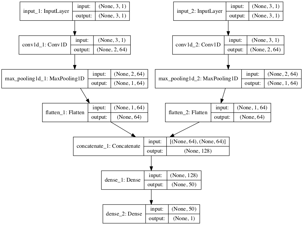
문제를 모델링하는 더 정교한 방법이 존재하는데, 각 input series는 별도의 CNN에 의해 처리될 수 있고, output sequence를 예측하기 전에 각 하위 모델의 output을 결합할 수 있습니다. 이를 multi-headed CNN model이라 하고, 모델링 중인 문제의 성능에 세부 사항들에 따라 더 많은 유연성을 제공하거나 더 나은 성능을 제공합니다. 예를 들면, 각 input series에 대해 filter map의 개수, kernel size와 같은 하위 모델을 다르게 구성할 수 있습니다. 이러한 유형의 모델은 Keras functional API에서 구현 가능합니다.
# first input model
visible1 = Input(shape=(n_steps, n_features))
cnn1 = Conv1D(filters=64, kernel_size=2, activation='relu')(visible1)
cnn1 = MaxPooling1D(pool_size=2)(cnn1)
cnn1 = Flatten()(cnn1)

# second input model
visible2 = Input(shape=(n_steps, n_features))
cnn2 = Conv1D(filters=64, kernel_size=2, activation='relu')(visible2)
cnn2 = MaxPooling1D(pool_size=2)(cnn2)
cnn2 = Flatten()(cnn2)

from keras.layers.merge import concatenate

# merge input models
merge = concatenate([cnn1, cnn2])
dense = Dense(50, activation='relu')(merge)
output = Dense(1)(dense)

model = Model(inputs=[visible1, visible2], outputs=output)
2개의 input model(하위 모델)을 만들었으므로 각 모델의 output을 output sequence를 예측하기 전에 해석할 수 있는 하나의 긴 벡터로 병합하게 됩니다. 다음 이미지는 각 레이어이 input, output shape을 포함하여 모델에 대한 도식을 보여줍니다.
이 모델은 리스트의 각 input times series를 하나의 모델의 input으로 넣습니다. 이를 위해 3D input data를 두 개의 개별 input data array로 분할합니다. 즉, 모양이 [7, 3, 2]인 하나의 배열에서 [7, 3, 1]인 두 개의 3D 배열로 분할하게 됩니다. (아래 그림 참고)
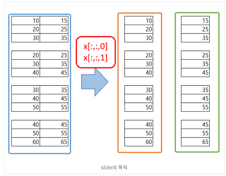
# one time series per head
n_features = 1

# separate input data
X1 = X[:, :, 0].reshape(X.shape[0], X.shape[1], n_features)
X2 = X[:, :, 1].reshape(X.shape[0], X.shape[1], n_features)

model = Model(inputs=[visible1, visible2], outputs=output)
model.compile(optimizer='adam', loss='mse')

# fit model
model.fit([X1, X2], y, epochs=1000, verbose=0)

# demonstrate prediction
x_input = array([[80, 85], [90, 95], [100, 105]])
x1 = x_input[:, 0].reshape((1, n_steps, n_features))
x2 = x_input[:, 1].reshape((1, n_steps, n_features))
yhat = model.predict([x1, x2], verbose=0)
print(yhat)
[[206.5997]]
새로운 관측치 [[80, 85], [90, 95], [100, 105]]에 대한 예측 값은 206.6임을 알 수 있습니다.
2.2 Multiple Parallel Series
Multiple Parallel Series는 여러 개의 병렬 시계열이 있고, 각각에 대해 값을 예측해야하는 경우입니다. (아래 그림 참고)
2.2.1 Data Preparation
[[ 10 15 25][ 20 25 45]
[ 30 35 65][ 40 45 85]
[ 50 55 105][ 60 65 125]
[ 70 75 145][ 80 85 165]
[ 90 95 185]]
앞 예제와 동일한 데이터가 주어졌을 때, 다음 step에서는 3개의 시계열 각각에 대한 값을 예측할 수 있고, 이를 multivariate forecasting 이라 합니다. 모델을 학습하기 위해서 데이터를 input/output sample으로 분할해야하고, 첫 번째 sample은 다음과 같습니다.
[input]
10, 15, 25
20, 25, 45
30, 35, 65
[output]
40, 45, 85
# multivariate output data prep
from numpy import array
from numpy import hstack

# split a multivariate sequence into samples
def split_sequences(sequences, n_steps):
    X, y = list(), list()
    for i in range(len(sequences)):
        # find the end of this pattern
        end_ix = i + n_steps
        # check if we are beyond the dataset
        if end_ix > len(sequences)-1:
            break
        # gather input and output parts of the pattern
        seq_x, seq_y = sequences[i:end_ix, :], sequences[end_ix, :]
        X.append(seq_x)
        y.append(seq_y)
    return array(X), array(y)

# define input sequence
in_seq1 = array([10, 20, 30, 40, 50, 60, 70, 80, 90])
in_seq2 = array([15, 25, 35, 45, 55, 65, 75, 85, 95])
out_seq = array([in_seq1[i]+in_seq2[i] for i in range(len(in_seq1))])

# convert to [rows, columns] structure
in_seq1 = in_seq1.reshape((len(in_seq1), 1))
in_seq2 = in_seq2.reshape((len(in_seq2), 1))
out_seq = out_seq.reshape((len(out_seq), 1))

# horizontally stack columns
dataset = hstack((in_seq1, in_seq2, out_seq))

# choose a number of time steps
n_steps = 3

# convert into input/output
X, y = split_sequences(dataset, n_steps)
print(X.shape, y.shape)

# summarize the data
for i in range(len(X)):
    print(X[i], y[i])
(6, 3, 3) (6, 3)
[[10 15 25]
[20 25 45]
[30 35 65]][40 45 85]
[[20 25 45]
[30 35 65]
[40 45 85]][ 50 55 105]
[[ 30 35 65]
[ 40 45 85]
[ 50 55 105]][ 60 65 125]
[[ 40 45 85]
[ 50 55 105]
[ 60 65 125]][ 70 75 145]
[[ 50 55 105]
[ 60 65 125]
[ 70 75 145]][ 80 85 165]
[[ 60 65 125]
[ 70 75 145]
[ 80 85 165]][ 90 95 185]
split_sequences() 함수는 time step에 대한 row와 column 당 하나의 시리즈가 있는 여러개의 병렬 시계열을 필요한 input/output shape으로 분할합니다. X의 shape은 3차원으로, (number of samples, number of time steps chosen per sample, number of parallel time series or features : (6,3,3))으로 구성됩니다. Y의 shape은 2차원으로, (number of samples, number of time variables per sample : (6,3))로 구성됩니다. 데이터는 각 샘플의 X, Y에 대해 3차원 input 및 2차원 output shape을 기대하는 1D CNN 모델에서 사용할 수 있습니다. 이 모델에서, input_shape 파라미터를 통해 input layer에 대한 time step의 수와 병렬 시계열을 지정합니다. 병렬 시계열의 수는 output layer에서 모델에 의해 예측할 값의 수 형식에 대해서도 사용됩니다. -> 즉, 3입니다.
2.2.2 CNN Model
# define model

from keras.models import Sequential
from keras.layers import Dense
from keras.layers import Flatten
from keras.layers.convolutional import Conv1D
from keras.layers.convolutional import MaxPooling1D

n_features = X.shape[2]

model = Sequential()
model.add(Conv1D(filters=64, kernel_size=2, activation='relu', input_shape=(n_steps, n_features)))
model.add(MaxPooling1D(pool_size=2))
model.add(Flatten())
model.add(Dense(50, activation='relu'))
model.add(Dense(n_features))
model.compile(optimizer='adam', loss='mse')

# fit model
model.fit(X, y, epochs=3000, verbose=0)

# demonstrate prediction
x_input = array([[70,75,145], [80,85,165], [90,95,185]])
x_input = x_input.reshape((1, n_steps, n_features))
yhat = model.predict(x_input, verbose=0)
print(yhat)
[[101.08318 106.739456 208.01721 ]]
각 시리즈에 대해 3 time step의 입력을 제공함으로써 3개의 병렬 시계열 각각 다음 값을 예측할 수 있습니다. single prediction을 위한 input shape은 [1,3,3] 이어야 합니다.(1 sample, 3 time steps, 3 features) 새로운 관측치 [[70,75,145], [80,85,165], [90,95,185]]에 대한 예측값은 [[101.08318 106.739456 208.01721 ]]임을 알 수 있습니다.
2.2.3 Multi-output CNN Model
multiple input series와 마찬가지로, 문제를 모델링하는 또 다른 방법이 존재합니다. 각 output series를 별도의 output CNN 모델에 의해 처리할 수 있는데, 이를 multi-output CNN model이라 합니다. keras functional API를 사용하여 케라스에서 정의 가능합니다. 첫 번째 input model을 1D CNN으로 정의할 수 있습니다.
from keras.layers import Input

# define model
visible = Input(shape=(n_steps, n_features))
cnn = Conv1D(filters=64, kernel_size=2, activation='relu')(visible)
cnn = MaxPooling1D(pool_size=2)(cnn)
cnn = Flatten()(cnn)
cnn = Dense(50, activation='relu')(cnn)
그 다음, 예측하고자 하는 3개의 시리즈 각각에 대해 하나의 output layer를 정의할 수 있고, 각 output submodel은 single time step을 예측합니다.
# define output 1
output1 = Dense(1)(cnn)
# define output 2
output2 = Dense(1)(cnn)
# define output 3
output3 = Dense(1)(cnn)
그 후 input layer와 output layer를 single model로 연결할 수 있습니다.
from keras.models import Model

# tie together
model = Model(inputs=visible, outputs=[output1, output2, output3])
model.compile(optimizer='adam', loss='mse')
model architecture를 명확히 하기 위해, 아래의 도식은 모델의 3개의 분리된 output layer와 각 레이어의 input 및 output shape을 명확하게 보여줍니다.
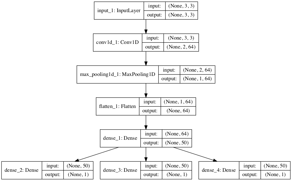
모델을 학습할 때, sample 당 별도의 output array가 필요하므로 shape [7,3]을 갖는 output training data를 shape [7,1]을 갖는 3개의 배열로 변환합니다.
# separate output
y1 = y[:, 0].reshape((y.shape[0], 1))
y2 = y[:, 1].reshape((y.shape[0], 1))
y3 = y[:, 2].reshape((y.shape[0], 1))

# fit model
model.fit(X, [y1,y2,y3], epochs=2000, verbose=0)

# demonstrate prediction
x_input = array([[70,75,145], [80,85,165], [90,95,185]])
x_input = x_input.reshape((1, n_steps, n_features))
yhat = model.predict(x_input, verbose=0)
print(yhat)
[array([[101.1715]], dtype=float32), array([[106.36812]], dtype=float32), array([[207.49104]], dtype=float32)]
새로운 관측치 [[70,75,145], [80,85,165], [90,95,185]]에 대한 예측값은 위의 결과와 같습니다.
3. Multi-Step CNN Models
실제로, 다른 output 변수를 나타내는 vector output 또는 하나의 변수에 대해 여러 time step을 나타내는 vector output을 예측하는 1D CNN 모델은 거의 차이가 없습니다. 그럼에도 불구하고, training data를 준비하는 방법에는 중요한 차이가 존재하는데, 이번 섹션에서는 vector model을 사용하여 multi-step 예측 모델을 간단히 구현해보도록 하겠습니다.
3.1 Data Preparation
one-step forcasting과 마찬가지로, multi-step 시계열 예측에 사용되는 시계열을 input과 output이 있는 sample로 분할해야 합니다. input과 output 구성요소는 모두 여러 time step으로 구성되며, 동일한 step 수를 가질 수도 있고 다른 step 수를 가질 수도 있습니다.
예를 들어, 일변량 시계열이 주어지면, 최근 3개의 time step을 이용하여 2개의 다음 time step을 예측할 수 있습니다. 첫번째 sample은 다음과 같습니다.
[input][10,20,30]
[output][40,50]
# split a univariate sequence into samples
def split_sequence(sequence, n_steps_in, n_steps_out):
    X, y = list(), list()
    for i in range(len(sequence)):
        # find the end of this pattern
        end_ix = i + n_steps_in
        out_end_ix = end_ix + n_steps_out
        # check if we are beyond the sequence
        if out_end_ix > len(sequence):
            break
        # gather input and output parts of the pattern
        seq_x, seq_y = sequence[i:end_ix], sequence[end_ix:out_end_ix]
        X.append(seq_x)
        y.append(seq_y)
    return array(X), array(y)
split_sequence() 함수는 이 동작을 구현하며, 일변량 시계열을 지정된 수의 input과 output의 time step을 가진 sample로 분할합니다.
# multi-step data preparation
from numpy import array

# define input sequence
raw_seq = [10, 20, 30, 40, 50, 60, 70, 80, 90]

# choose a number of time steps
n_steps_in, n_steps_out = 3, 2

# split into samples
X, y = split_sequence(raw_seq, n_steps_in, n_steps_out)

# summarize the data
for i in range(len(X)):
    print(X[i], y[i])
[10 20 30][40 50]
[20 30 40][50 60]
[30 40 50][60 70]
[40 50 60][70 80]
[50 60 70][80 90]
multi-step forecasting을 위한 데이터(x,y)를 준비했으므로 이를 학습할 수 있는 1D CNN 모델을 살펴보도록 하겠습니다.
3.2 Vector Output Model
1D CNN은 multi-step 예측으로 해석될 수 있는 vector를 직접 출력할 수 있습니다. 이 접근법은 이전 섹션에서 볼 수 있었는데, 각 output 시계열의 one time step이 vector로 예측되었습니다. 이전 섹션의 일변량 데이터에 대한 1D CNN 모델과 마찬가지로, sample을 3차원으로 reshape 해주어야 하며 현재 case는 하나의 feature를 가지게 됩니다.
# reshape from [samples, timesteps] into [samples, timesteps, features]
n_features = 1
X = X.reshape((X.shape[0], X.shape[1], n_features))
X
array([[[10],[20],[30]],
[[20],[30],[40]],
[[30],[40],[50]],
[[40],[50],[60]],
[[50],[60],[70]]])
# define model
model = Sequential()
model.add(Conv1D(filters=64, kernel_size=2, activation='relu', input_shape=(n_steps_in, n_features)))
model.add(MaxPooling1D(pool_size=2))
model.add(Flatten())
model.add(Dense(50, activation='relu'))
model.add(Dense(n_steps_out))
model.compile(optimizer='adam', loss='mse')

# fit model
model.fit(X, y, epochs=2000, verbose=0)

# demonstrate prediction
x_input = array([70, 80, 90])
x_input = x_input.reshape((1, n_steps_in, n_features))
yhat = model.predict(x_input, verbose=0)
print(yhat)
[[103.26184 115.395706]]
n_steps_in과 n_steps_out 변수는 각각 input과 output의 step 수를 의미하며, 이를 이용해 multi-step 시계열 예측 모델을 정의할 수 있습니다. 예측을 수행할 때 input data의 single sample shape은 [1,3,1]이 되어야 합니다. (1 sample, 3 time steps of the input, single feature). 새로운 관측치 [70, 80, 90]에 대한 예측값은 위와 같습니다.
4. Multivariate Multi-Step CNN Models
Multivariate multi-step CNN model (다변량 다단계)는 2가지로 나눌 수 있습니다.
1) Multiple Input Multi-Step Output
2) Multiple Parallel Input and Multi-Step Output
4.1 Multiple Input Multi-Step Output (다중 입력 / 다단계 출력)
output series가 개별적이지만 input 시계열에 따라 달라지며 output series에 여러 time step가 필요한 multivariate 다변량 시계열 예측 문제가 존재합니다.
예를 들어, 이전 섹션의 다변량 시계열 데이터셋에서 output 시계열의 2 time step을 예측하기 위해 2개의 input 시계열 각각에 대한 3가지의 이전 time step을 이용하는 것입니다. training dataset의 첫 번째 sample은 다음과 같습니다.
[input]
10, 15
20, 25
30, 35
[output]
65
85
4.1.1 Data Preparation
# split a multivariate sequence into samples
def split_sequences(sequences, n_steps_in, n_steps_out):
	X, y = list(), list()
	for i in range(len(sequences)):
		# find the end of this pattern
		end_ix = i + n_steps_in
		out_end_ix = end_ix + n_steps_out-1
		# check if we are beyond the dataset
		if out_end_ix > len(sequences):
			break
		# gather input and output parts of the pattern
		seq_x, seq_y = sequences[i:end_ix, :-1], sequences[end_ix-1:out_end_ix, -1]
		X.append(seq_x)
		y.append(seq_y)
	return array(X), array(y)

# multivariate multi-step data preparation
from numpy import array
from numpy import hstack

# define input sequence
in_seq1 = array([10, 20, 30, 40, 50, 60, 70, 80, 90])
in_seq2 = array([15, 25, 35, 45, 55, 65, 75, 85, 95])
out_seq = array([in_seq1[i]+in_seq2[i] for i in range(len(in_seq1))])

# convert to [rows, columns] structure
in_seq1 = in_seq1.reshape((len(in_seq1), 1))
in_seq2 = in_seq2.reshape((len(in_seq2), 1))
out_seq = out_seq.reshape((len(out_seq), 1))

# horizontally stack columns
dataset = hstack((in_seq1, in_seq2, out_seq))

# choose a number of time steps
n_steps_in, n_steps_out = 3, 2

# convert into input/output
X, y = split_sequences(dataset, n_steps_in, n_steps_out)
print(X.shape, y.shape)

# summarize the data
for i in range(len(X)):
	print(X[i], y[i])
(6, 3, 2) (6, 2)
[[10 15]
[20 25]
[30 35]][65 85]
[[20 25]
[30 35]
[40 45]][ 85 105]
[[30 35]
[40 45]
[50 55]][105 125]
[[40 45]
[50 55]
[60 65]][125 145]
[[50 55]
[60 65]
[70 75]][145 165]
[[60 65]
[70 75]
[80 85]][165 185]
training data의 shape을 보면 sample의 input shape은 3차원이며, 6개의 sample, 3개의 time step, 2개의 input 시계열에 대한 변수로 이루어져 있습니다.
sample의 output shape은 2차원이며, 6개의 sample, 예측될 각 sample에 대한 2개의 time step으로 구성됩니다.
4.1.2 Vector Output Model
이제 multi-step prediction을 위한 1D CNN 모델을 개발할 수 있고, vector output model을 구현해보겠습니다.
# the dataset knows the number of features, e.g. 2
n_features = X.shape[2]

# define model
model = Sequential()
model.add(Conv1D(filters=64, kernel_size=2, activation='relu', input_shape=(n_steps_in, n_features)))
model.add(MaxPooling1D(pool_size=2))
model.add(Flatten())
model.add(Dense(50, activation='relu'))
model.add(Dense(n_steps_out))
model.compile(optimizer='adam', loss='mse')

# fit model
model.fit(X, y, epochs=2000, verbose=0)

# demonstrate prediction
x_input = array([[70, 75], [80, 85], [90, 95]])
x_input = x_input.reshape((1, n_steps_in, n_features))
yhat = model.predict(x_input, verbose=0)
print(yhat)
[[185.32578 206.12723]]
새로운 관측치 [[70, 75], [80, 85], [90, 95]]에 대한 관측값은 위와 같습니다.
4.2 Multiple Parallel Input and Multi-Step Output
병렬 시계열 문제는 각 시계열의 여러 time step를 예측할 수 있어야 합니다.
예를 들어, 이전 섹션의 다변량 시계열 데이터셋에서 3개의 시계열 각각의 마지막 3 time step을 모델의 input으로 사용할 수 있고, 3개의 시계열 각각에 대한 다음 time step을 output으로 예측할 수 있습니다. training dataset의 첫 번째 sample은 다음과 같습니다.
[input]
10, 15, 25
20, 25, 45
30, 35, 65
[output]
40, 45, 85
50, 55, 105
4.2.1 Data Preparation
# split a multivariate sequence into samples
def split_sequences(sequences, n_steps_in, n_steps_out):
	X, y = list(), list()
	for i in range(len(sequences)):
		# find the end of this pattern
		end_ix = i + n_steps_in
		out_end_ix = end_ix + n_steps_out
		# check if we are beyond the dataset
		if out_end_ix > len(sequences):
			break
		# gather input and output parts of the pattern
		seq_x, seq_y = sequences[i:end_ix, :], sequences[end_ix:out_end_ix, :]
		X.append(seq_x)
		y.append(seq_y)
	return array(X), array(y)

# define input sequence
in_seq1 = array([10, 20, 30, 40, 50, 60, 70, 80, 90])
in_seq2 = array([15, 25, 35, 45, 55, 65, 75, 85, 95])
out_seq = array([in_seq1[i]+in_seq2[i] for i in range(len(in_seq1))])

# convert to [rows, columns] structure
in_seq1 = in_seq1.reshape((len(in_seq1), 1))
in_seq2 = in_seq2.reshape((len(in_seq2), 1))
out_seq = out_seq.reshape((len(out_seq), 1))

# horizontally stack columns
dataset = hstack((in_seq1, in_seq2, out_seq))

# choose a number of time steps
n_steps_in, n_steps_out = 3, 2

# convert into input/output
X, y = split_sequences(dataset, n_steps_in, n_steps_out)
print(X.shape, y.shape)

# summarize the data
for i in range(len(X)):
	print(X[i], y[i])
(5, 3, 3) (5, 2, 3)
[[10 15 25][20 25 45]
[30 35 65]] [[ 40 45 85][ 50 55 105]]
[[20 25 45][30 35 65]
[40 45 85]] [[ 50 55 105][ 60 65 125]]
[[ 30 35 65][ 40 45 85]
[ 50 55 105]] [[ 60 65 125][ 70 75 145]]
[[ 40 45 85][ 50 55 105]
[ 60 65 125]] [[ 70 75 145][ 80 85 165]]
[[ 50 55 105][ 60 65 125]
[ 70 75 145]] [[ 80 85 165][ 90 95 185]]
우리는 데이터셋의 input과 output이 각각 3차원임을 알 수 있습니다.(number of samples, time steps, variables or parallel time series)
4.2.2 Vector Output Model
이제 이 데이터셋에 대한 1D CNN 모델을 개발할 수 있고, vector output 모델을 사용합니다. 모델을 학습시키기 위해 각 sample의 output 부분의 3차원 구조를 flatten하게 만들어야 합니다. 즉, 각 시리즈에 대해 2 step을 예측하는 대신 모델이 학습되고, 6개의 벡터를 직접 예측할 것으로 기대됩니다.
# flatten output
n_output = y.shape[1] * y.shape[2]
y = y.reshape((y.shape[0], n_output))

# the dataset knows the number of features, e.g. 2
n_features = X.shape[2]

# define model
model = Sequential()
model.add(Conv1D(filters=64, kernel_size=2, activation='relu', input_shape=(n_steps_in, n_features)))
model.add(MaxPooling1D(pool_size=2))
model.add(Flatten())
model.add(Dense(50, activation='relu'))
model.add(Dense(n_output))
model.compile(optimizer='adam', loss='mse')

# fit model
model.fit(X, y, epochs=7000, verbose=0)

# demonstrate prediction
x_input = array([[60, 65, 125], [70, 75, 145], [80, 85, 165]])
x_input = x_input.reshape((1, n_steps_in, n_features))
yhat = model.predict(x_input, verbose=0)
print(yhat)
[[ 91.57259 97.15711 188.71162 103.26472 108.2695 210.43442]]
새로운 관측치 [[60, 65, 125], [70, 75, 145], [80, 85, 165]]에 대한 예측값은 위와 같습니다.
5. References
https://machinelearningmastery.com/how-to-develop-convolutional-neural-network-models-for-time-series-forecasting/
https://mellowlee.tistory.com/entry/ML-Multiple-Input-Series-Multi-headed-CNN-Model
https://mellowlee.tistory.com/entry/ML-Multiple-Parallel-Series
https://machinelearningmastery.com/using-cnn-for-financial-time-series-prediction/
https://www.tensorflow.org/tutorials/structured_data/time_series?hl=ko#단일_스텝_모델
https://pseudo-lab.github.io/Tutorial-Book/chapters/time-series/Ch5-CNN-LSTM.html
https://gmnam.tistory.com/274