Computer Networking Final Term

Credit: 3
Status: In progress

시험 범위 챕터 3 ~ 5 (일부 제외되어 있음)

챕터 3 : Transport Layer

챕터 4 : Network Layer : Data Plane

챕터 5 : Network Layer : Control Plane

챕터 4 → 챕터 5 → 3 장 순서로 공부 → 책 내용 (extra 시험범위)

Quick access

[정보통신기술용어해설]

[네트워크] 4.2 Internet Protocol

Selective Repeat / Go Back N

Ch.4 Network Layer: Data Plane

• Sender : encapsulates segments into datagrams, passes to link layer

• Receiver : delivers segments to transport layer protocol

• forwarding : router’s input link → appropriate router output link

• routing : source → destination

Data plane

local, per-router function

Control plane

Network-wide logic

1. trainditonal routing algorithms : implemented in routers
2. software-defined networking (SDN) : implemeted in
   (remote) severs

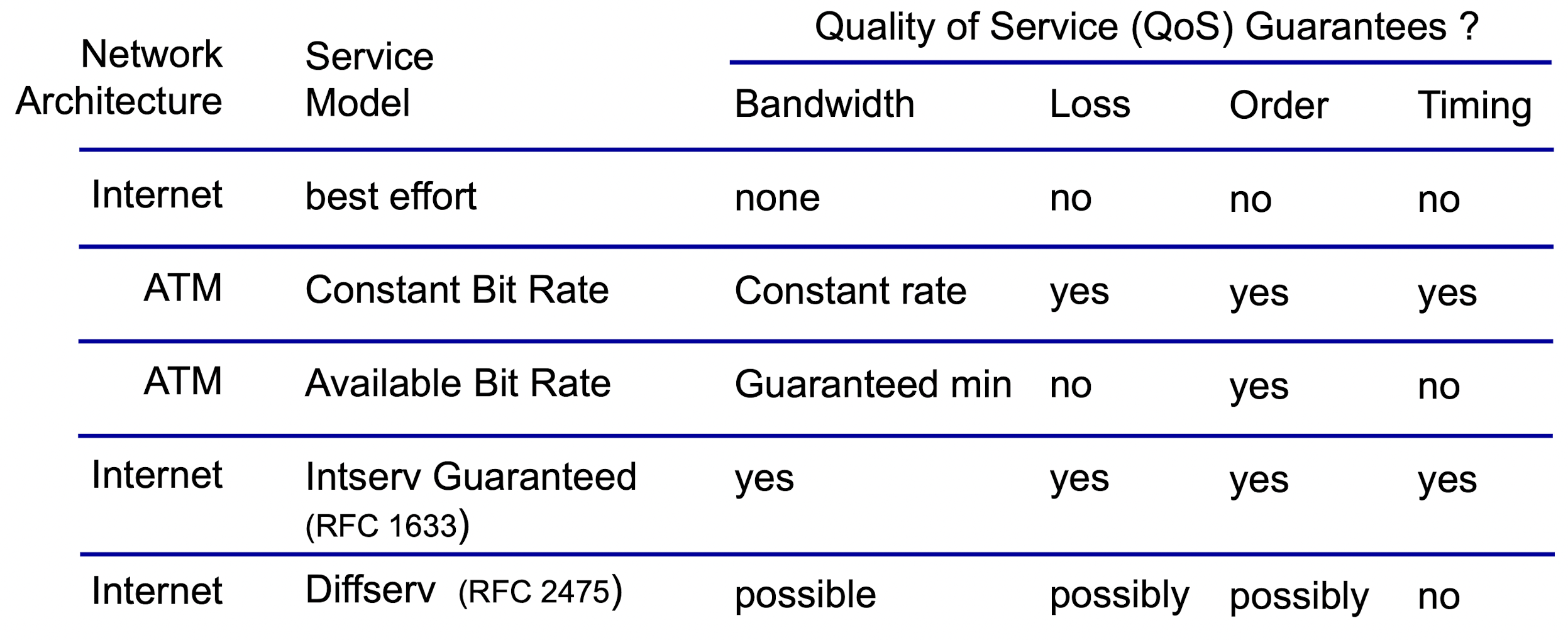
Network-layer service model

Internet “best effort” service model

No guarantees on:

1. successful datagram delivery to destination
2. timing or order of delivery
3. bandwidth available to end-end flow

Reflections onf best-effort service

• Simplicity of mechnism has allowed internet to be widely deployed adopted
• Sufficient provisiong(공급) of bandwidth allows performance of real-time applications (e.g., interactive voice, video) to be “good enough” for “most of the time”
• Replicated, application-layer distributed services (datacenters, content distribution networks) connecting close to clients’ networks, allow services to be provided from multiple locations
• congestion control of “elastic” services helps

It’s hard to argu with success of best-effort service model

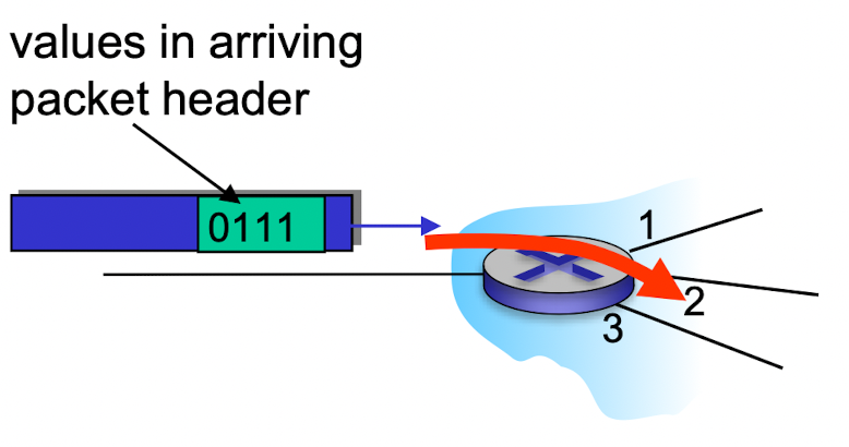
Input port functions

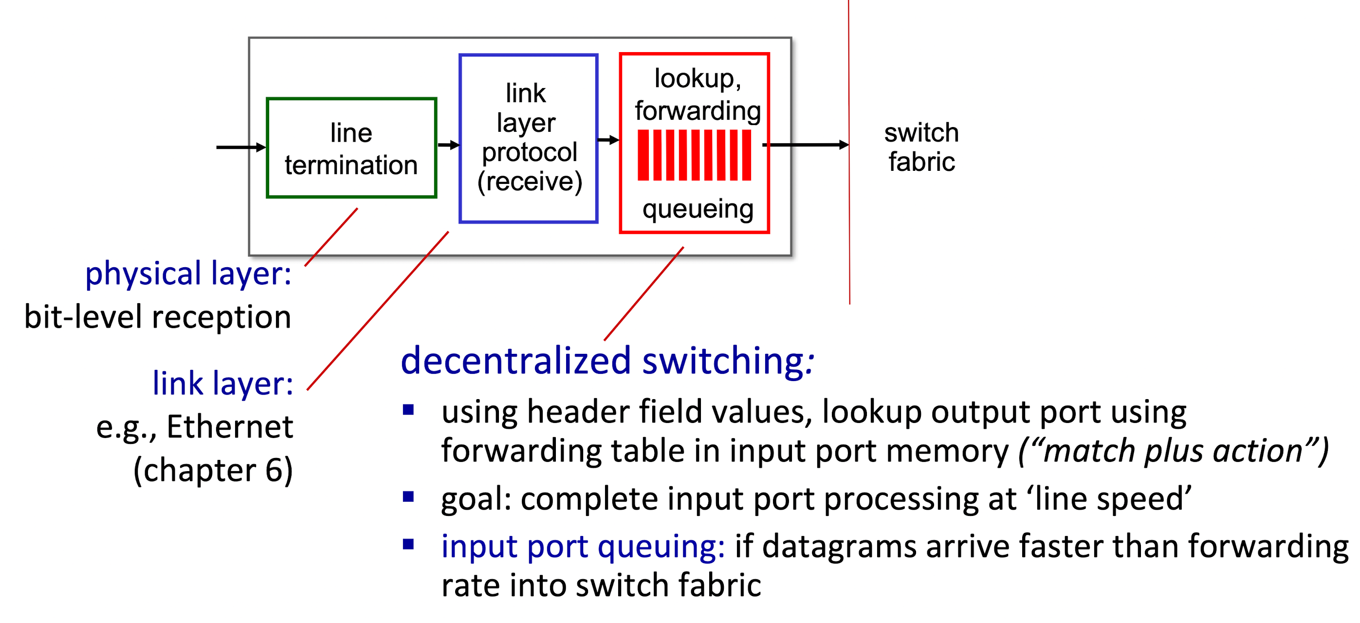
• destination-based forwarding : forward based only on destination IP address (traditional), simpler and afforadable
• generalized forwarding (SDN) : forward based on any set of header filed values, complicated and expensive

Longest prefix matching

When looking for forwarding table entry for given destination address, use longest address prefix that matches destination address.

Switching fabrics

transfer packet from input link to appropriate output link

swithcing rate : rate at which packets can be tranfer from inputs to outputs

• often measured as multiple of input/output line rate
• N inputs: switching rate N times line rate desirable

Three major types of switching fabrics

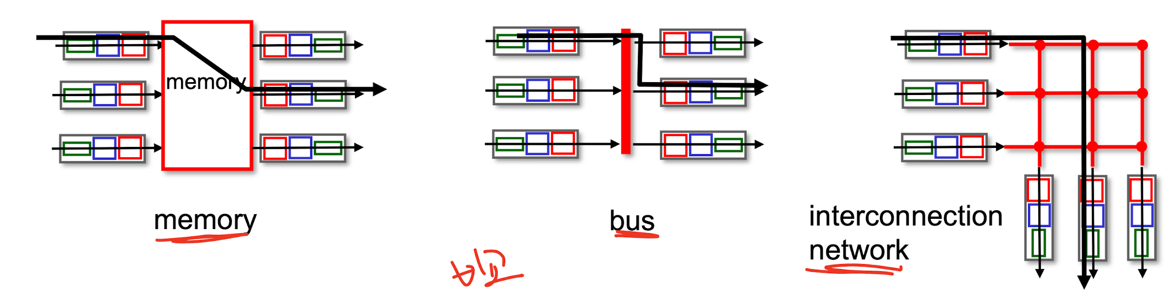
1. Memory

First generation routers:

Memory가 input port 와 output port 사이의 중간지점이다.

Speed limited by memory bandwidth (2 bus crossing per datagram)

2. Bus

Datagram goes direct from input port memory to output port memory via a shared bus

bus connection : switching speed limited by bus badnwidth

32 Gbps bus, Cisco 5600 : sufficien4t speed for access routers

3. Interconnection (=Crossbar, clos networks)

Interconnection nets initially developed to connect processor in multiprocessor

If bus speed is R, this switch can get 3R data through

Crosspoint : can be open and closed by switch fabric controller

Note that : if two packets from two different input ports are destined to the same output port, then on will have to wait at the input, since only one packet can be sent over any given bus at time.

More sophisticated interconnection networks use ****multiple stages**** of swithcing

Allow **packets from different input port** to proceed towards the ****same output port at the same time**** through the switching fabric.

Input port queuing

queueing **delay** and **loss** due to input **buffer** overflow !

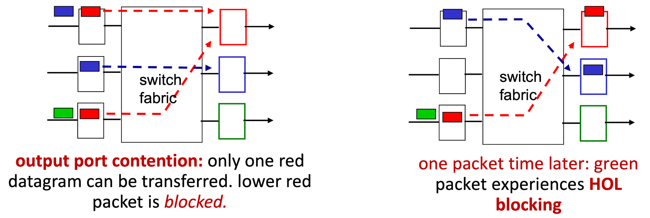
Output port queuing

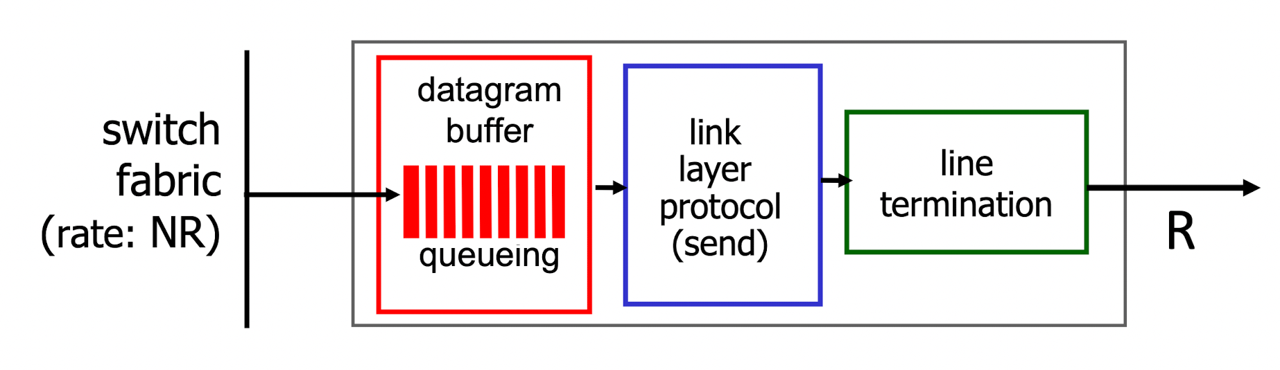
Buffering required when datagrams arrive from fabric faster than link transmission rate

Three things to decide here

1. How much buffering
2. Drop policy: which datagrams to drop if no free buffers? → datagrams can be lost due to congestion, lack of buffers
3. Scheduling disciplnie(규율) choose among queued datagrams for transmission → Priority scheduling : who gets best performance, network neutrality

with N flows, C link capacity, buffering equal to

$Average\;buffering\;=\frac{RTT \cdot C}{\sqrt{N}}$

해석 하면 : RTT (네트워크 사이즈) * C (output buffer에 물린 link capacity) / √N (TCP Conn. 개수)

Buffer Management : Drop Policy

Drop : which packet to add, drop when buffers are full / 종류 : tail drop, priority drop

marking : whcih packets to mark to signal congestion

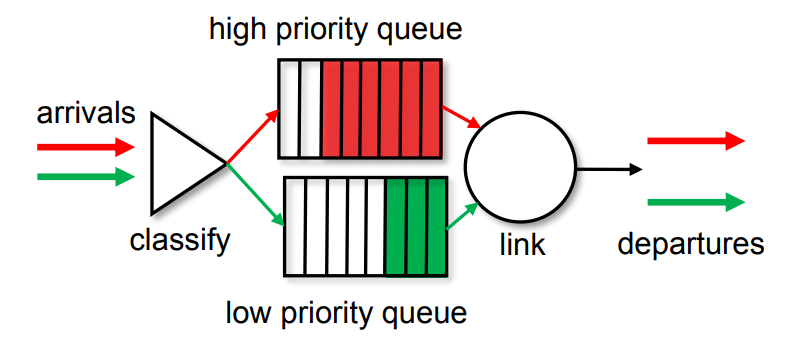
Buffer Management : Packet Scheduling : FCFS

packet scheduling : deciding which packet to send next on link

• first come, first served
• priority
  

• round robin
  • Arriving traffic classified, queued by class
    • any header fields can be used for classification
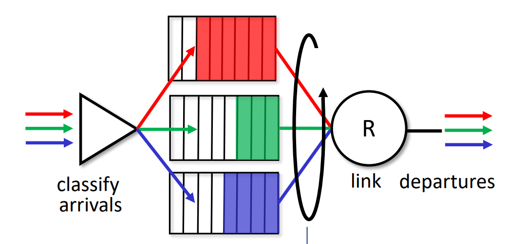
  • server cyclically, repeatedly scans class quees, sending one complete packet from each class in turn

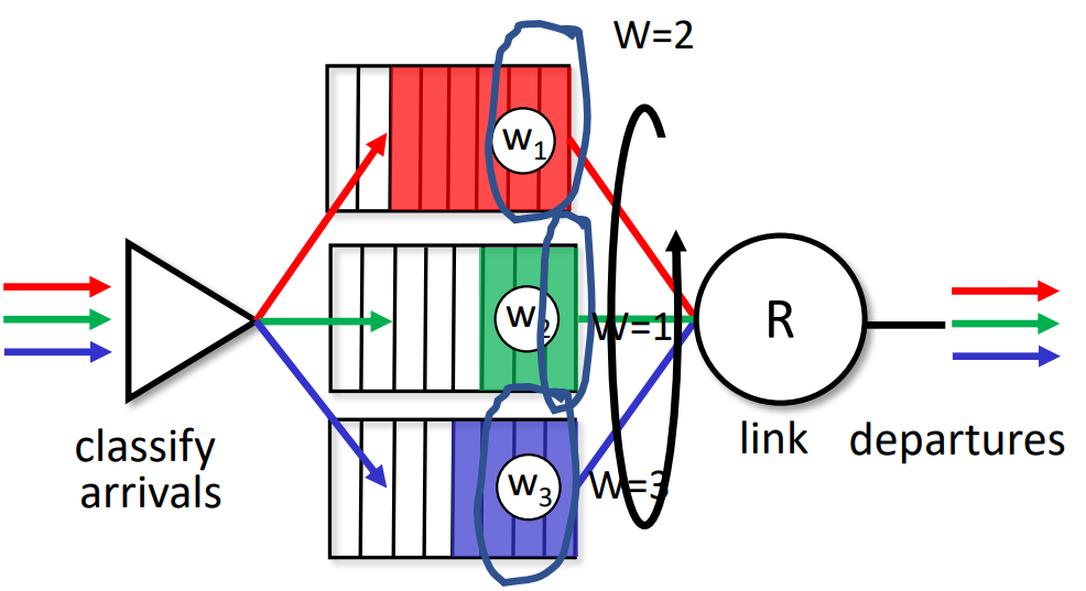
• weighted fair(≠ 공평한, = 규칙에 따른) queueing
  • generalized Round Robin
  • each class, i, has weight, wi, and gets weighted amount of service in each cycle $\frac{w_i}{\sum{j}w_j}$
  • minimum bandwidth guarantee (per-traffic-class)
    

Internet Protocol (IP)

IP Datagram format

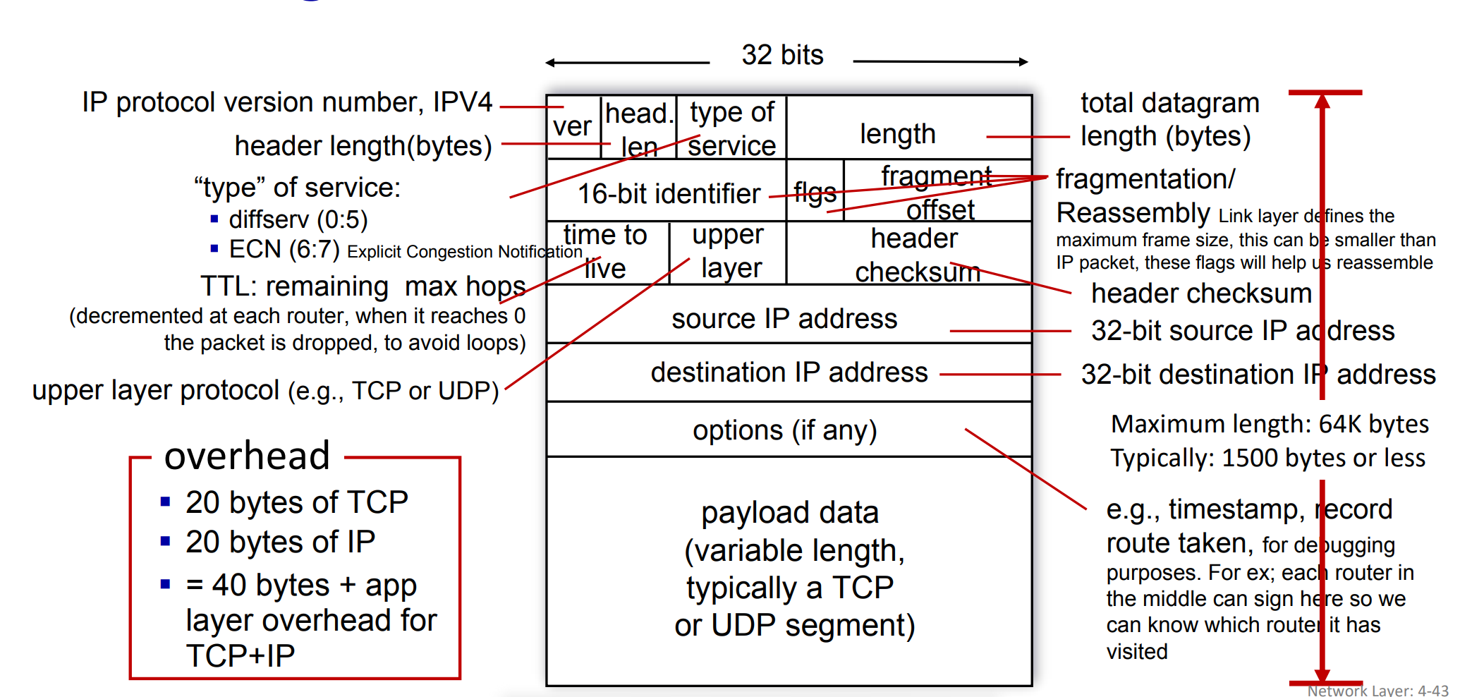
• head length : 주로 network 엔지니어들이 개발할 때 테스팅 용 옵션, 전형적인 IP Datagram의 헤더에 length는 TCP와 동일한 20bytes. 따라서 TCP & IP 를 사용하는 메세지는 기본적으로 40bytes의 오버헤드를 가짐

IPv4 fragmentation, reassembly

각 network link별로 MTU (Maximum Transmission unit = R) 상이함 → 각 라우터에서 다음 link의 MTU 보다 현제 datagram의 크기가 크면 쪼개서 보내야함. 즉 들어오는 R보다 나가는 R이 작은 경우

Reassembly는 final destination “host”에서만 하지 중간 router에서는 하지 않는다.

이유

• 각각의 sub packet들은 지나가는 경로가 다 다르기 때문에 이론 상 한 라우터로 간다는 보장이없음
• 맨 마지막에 router에서 합치는 것은 internet의 철학인 core network는 가능한 복잡한 일을 안 하고, simple하게 빨리 deliver하는 것이 목표. 복잡한 것은 host에 위배

fragmentation 시에는 헤더 (20byte)는 똑같이 복사되어 각 서브 패킷에 붙음

vs IPv6

IP version 6에서는 애초에 fragmentation하지 않는다 → 일단 전송하고 만약 MTU 초과 시, 호스트 단에서 fragmentation을 수행하여 다시 보냄

Subnets

device interfaces that can physically reach each other ****without passing through an intervening router****

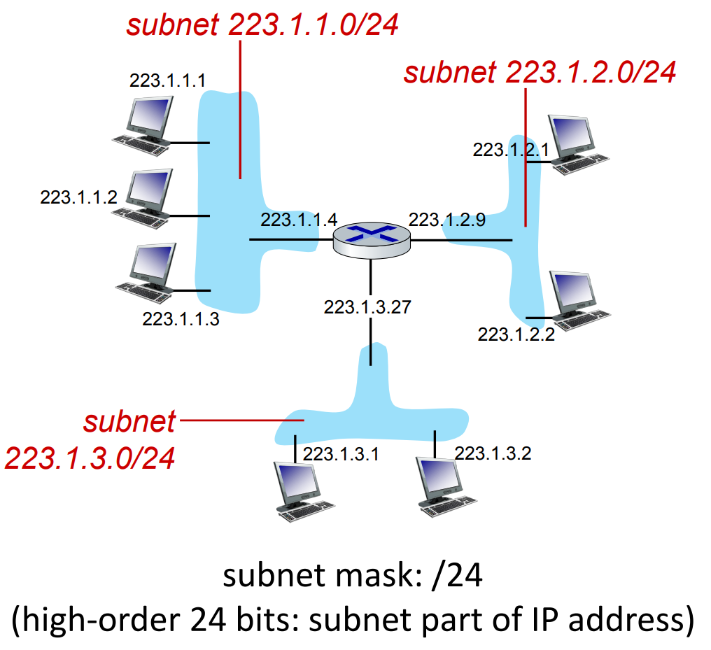
where are the subnets?

what are the /24 subnet address?

CIDR

CIDR : Classless InterDomain Routing

subnet portion of address of arbitrary length

address format : **a.b.c.d/x,** where x is # bits in subnet portion of address

[네트워크] CIDR이란?(사이더 란?)

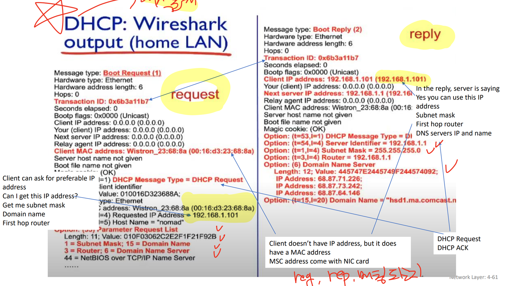
DHCP client-server scenario

well-known port 사용

server : 67번 포트

client : 68번 포트

src : source (출발지)

dest : destination (도착지)

시나리오 순서

1. DHCP discover : clinet가 우선 broadcast (port # 67)
2. DHCP offer : DHCP 서버가 포트 68번으로 후보 ip address를 broad cast
3. DHCP request : client가 할당된 ip를 사용하겠다고 67번 포트로 broad cast
4. DHCP ACK : 이 시점 부터 서버가 해당 clinet에게 ip 주소를 할당, broadcast로 응답을 보냄

→ 메세지를 주고 받을 때 끝까지 broadcast를 사용

NAT : netweork address translation

NAT: all devices in local network share just one IPv4 address as far as outside world is concerned

어떻게 바꿀 것이냐? local network를 떠나 Internet으로 가는 애들은 이 주소를 달고 갈 수 없기 때문에 공식적인 IP주소를 딱 하나만 받아(138.76.29.7) 나갈 때 무조건 이 주소를 대표로 바뀌어서 나감.

다 똑같은 주소로 나가면 어떻게 구별? 내가 가진 라우터가 NAPT를 지원하여(middle ware의 부가기능) port로 구별을 시킴

사용이유

• 모든 IP-capable device는 public routable IP address가 필요하다.
• IP에게 너무 많은 범위의 IP를 받을 필요가 없고 just one IP address for all devices가 필요할 때
• 주소가 노출이 안 되니 security 보장, 공격을 받지 않을 수 있음.
• 내 local network 안에서 device의 주소를 마음껏 바꿀 수 있고, 상위 ISP에게 알려줄 필요도 없음.

NAT vs IPv6

NAT : 사설 ip를 사용하기 때문에 ip가 노출되지 않아 보안에 강하다.

IPv6 : NAT는 이를 수행하는 장비가 필요 하지만 IPv6는 필요하지 않다. QoS 보장, 무결성 보장

CH 5. Network Layer : Control Plane

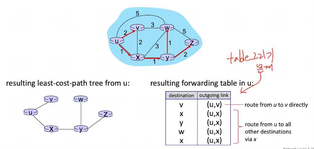
Dijstra’s algorithm

example

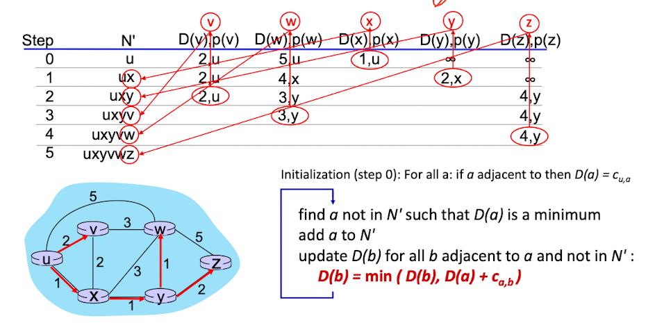
Algorithm complexity : n nodes

• each of n iteration : need to check all nodes, w, not in N
• n(n+1)/2 comparisons : $**O(n^2)**$ complexity
• more efficient implementation possible : $O(nlogn)$

Message complexity:

• each router must broadcast its link state information to other n routers
• efficient broadcast alorithms : $O(n)$ link crossing to disseminate a broadcast message from one source
• each router’s message corsses $O(n)$ links : overall message complexity : $O(n^2)$

Problem of Dijstra’s algorithm

Route oscillations problem

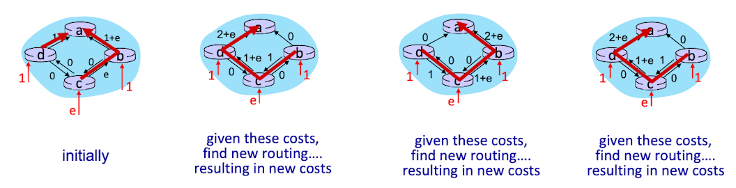
① 링크 비용 = 전송되는 트래픽 양

② 초기에는 시계반대방향 경로 선택

• D->A, C->B->A

③ 링크 상태 알고리즘을 한 번 더 수행하면 시계방향 선택

• B->C->D->A

④ 다시 수행하면 시계반대방향, 또 다시 수행하면 시계방향 경로를 선택하여 진동

Distnace vector algorithm

iterative, asynchronous

distributed, self-stopping

lonk cost changes:

node detects local link cost change

“bad news travels slow” - count-to-infinity problem

Comparison of LS (Link state = Dijkstra) and DV (Distance vector) algorithms

	LS	DV
message complexity	n routers, O(n^2) messages sent	exchange between neighbors; convergence time varies
speed of convergence	O(n^2) algorithm, O(n^2) messages → may have oscillations	convergence time varies; may have routing loops; count-to-infinity problem
robustness	router can advertise incorrect link cost; each router computes only its own table	DV router can advertise incorrect path cost : black-holing; each router’s table used by others: error propagate thru network

CH 3. Transport Layer

message 단위 : segment

logical communication between **processes**

multiplexing : handle data from multiple sockets, add transport header (위 → 아래, sender)

demultiplexing : use header info to deliver recieved segments to correct socket (아래 → 위, receiver)

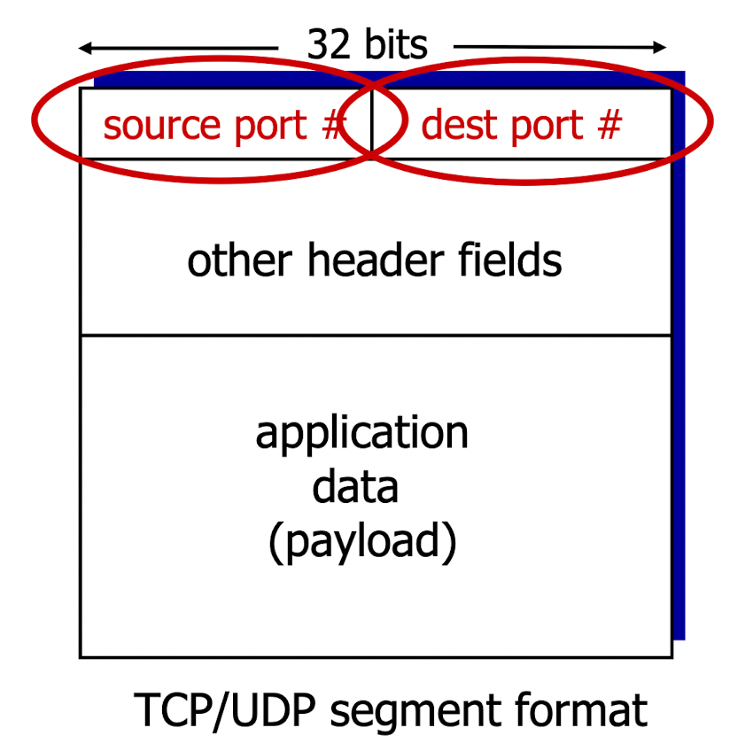
TCP demultiplexing by 4 tuple:

1. source IP address
2. source port number
3. dest IP address
4. dest port number

UDP : User Datagram Protocol

• no connection establishment
• small header size
• no congestion control

UDP segment header

UDP demultiplexing using destination port number (only)

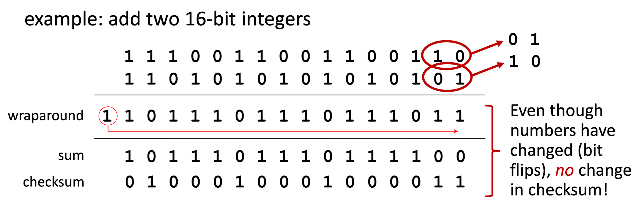
checksum

Principles of reliable data transfer

rdt 1.0 : 완벽하게 신뢰적인 채널 상에서의 신뢰적인 데이터 전송

기본적인 명령어

송신 측

• rdt_sed(data) : 이벤트에 의해 상위 계층으로 부터 데이터를 받음
• packet=make_pkt(data) 이벤트에 의해 데이터를 포함하는 패킷 생성
• udt_send(packet) 이벤트에 의해 패킷을 채널로 내려보내며 송신

수신 측

• rdt_rcv(packet) 이벤트에 의해 하위 채널로부터 패킷을 수신
• extract(packet, data) 이벤트에 의해 패킷으로부터 데이터를 추출
• deliver_data(data) 이벤트에 의헤 데이터를 상위 계층으로 전달

rdt 2.0 : 비트 오류가 있는 채널 상에서의 신뢰적인 데이터 전송

재전송을 기반으로 하는 신뢰적인 프로토콜을 자동재전송요구 프로토콜인 ARQ(Automatic Repeat reQuest) 사용

ARQ의 기능

• 오류 검출 : 체크섬 필드를 이용하여 비트 오류 검출
• 수신자 피드백 : ACK, NAK으로 피드백
• 재전송 : NAK일 때 재전송

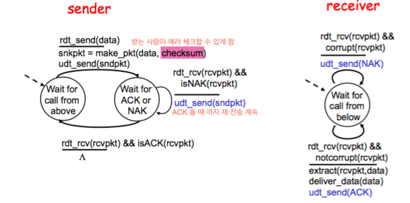
이 때 송신 측이 ACK 또는 NAK를 기다리는 오른쪽 상태에 있는 중에는 상위 계층으로부터 더 이상의 데이터를 전달받을수 없음 → Stop-and-Wait 프로토콜

치명적인 결함 : ACK/NAK 패킷의 손상가능성을 무시함 → 패킷에 순서번호 (sequence number)를 붙여서 해결 함(rdt 2.1)

rdt2.1, 2.2 : rdt 2.0의 수정버전

rdt2,1 : sequence number

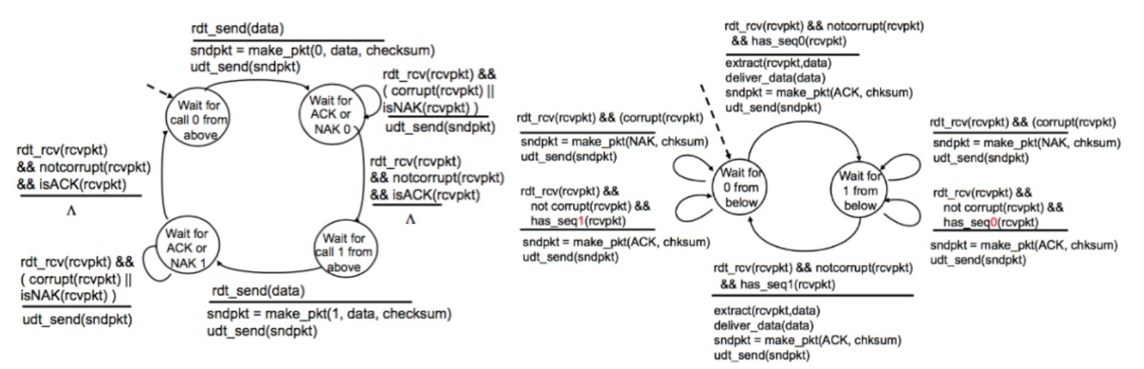
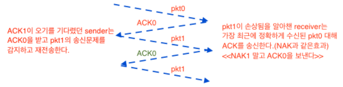
rdt 2.2 : NAK를 사용하지 않고 ACK만 사용하는 모델

NAK 대신에, 가장 최근에 잘 받은 패킷에 대한 ACK를 보냄으로써 NAK를 보내는 것과 동일한 효과를 얻을 수 있음

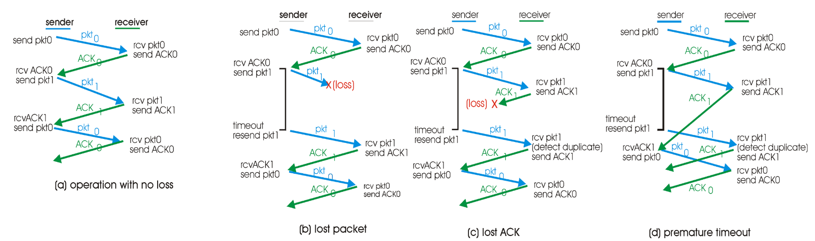
rdt3.0 : 비트손상과 함께 패킷을 손실하는 모델

어떻게 패킷손실을 검출하며, 패킷 손실이 발생하였을 때 어떤 핸동을 해야하는지 중요 → 체크섬, sequence number, ACK

패킷 손실의 검출을 Timer로 진행

rdt 3.0은 기능적으로 매우 정확하지만, 오늘날의 고속 네트워크에서 stop-and-wait 방식이므로 만족스러운 성능을 보여주지 못함

예시)

RTT = 30msec

전송률 R = 1Gbps (10^9)

패킷 크기 (L) = 헤더와 데이터를 포함하여 패킷 당 1000byte (8000bit)

패킷 전송 시간은?

즉, 8마이크로 sec 동안 송신측은 8000비트의 첫 비트 부터 마지막 비트 까지 수신측으로 보냄.

보낸 패킷들은 15msec(RTT/2) 이동하며, 수신측이 바로 ACK를 보낸다는 가정 하에 또 다른 15msec 후에 ACK가 송신 측으로 도착하기 때문에, 결국 송신 측은 30.008msec 후에 ACK받음

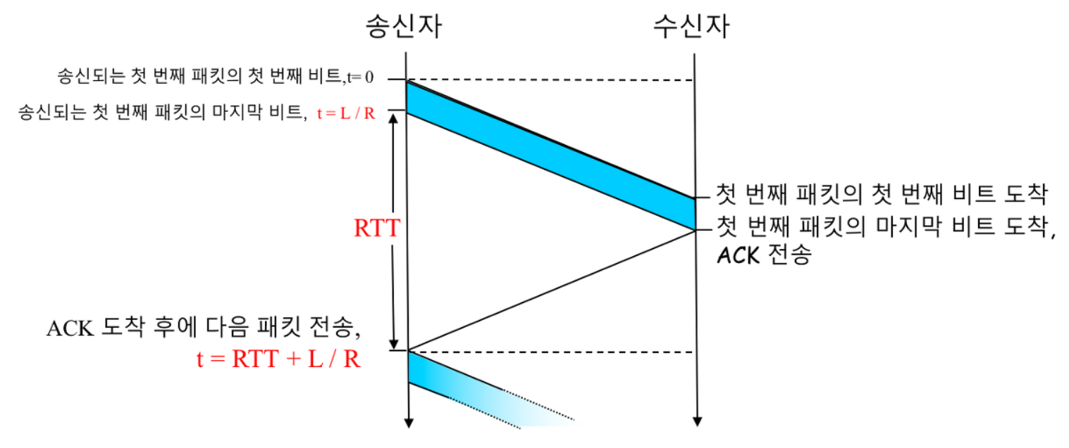
즉, 30.008msec 동안 송신측은 데이터 전송에 0.008msec만 사용 하였음.

따라서 이용률이 매우 낮다.

이에 대한 해결방안 : Pipelining

ACK를 기다리지 않고, 여러 패킷을 전송하는 방법

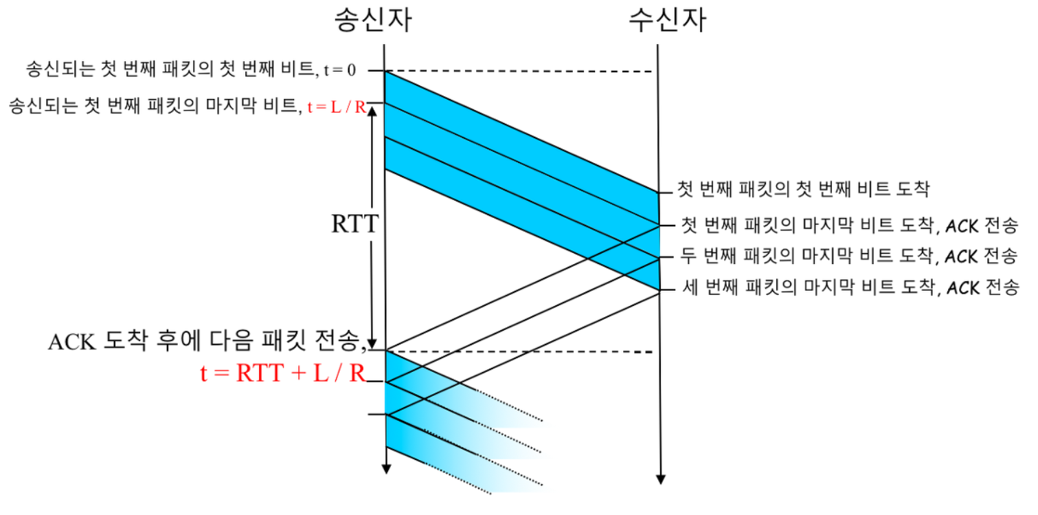
하지만 다음과 같은 사항을 고려해야함

• sequence number 범위의 증가 : 여러 패킷을 보낼 수 있게 됨으로써 0과 1로만으로는 부족
• 버퍼의 필요 : 송신 측과 수신 측은 여러 패킷 이상을 담을 수 있는 버퍼가 필요
• 파이프라인 오류 회복 방법 : 파이프라인에서 패킷 손실과 지연 패킷에 대한 처리방식이 필요

이러한 고려사항들을 만족시키기 위해 GBN(Go-Back-N, N부터 반복)과 SR(Selective Repeat, 선택적 반복) 프로토콜이 나타남

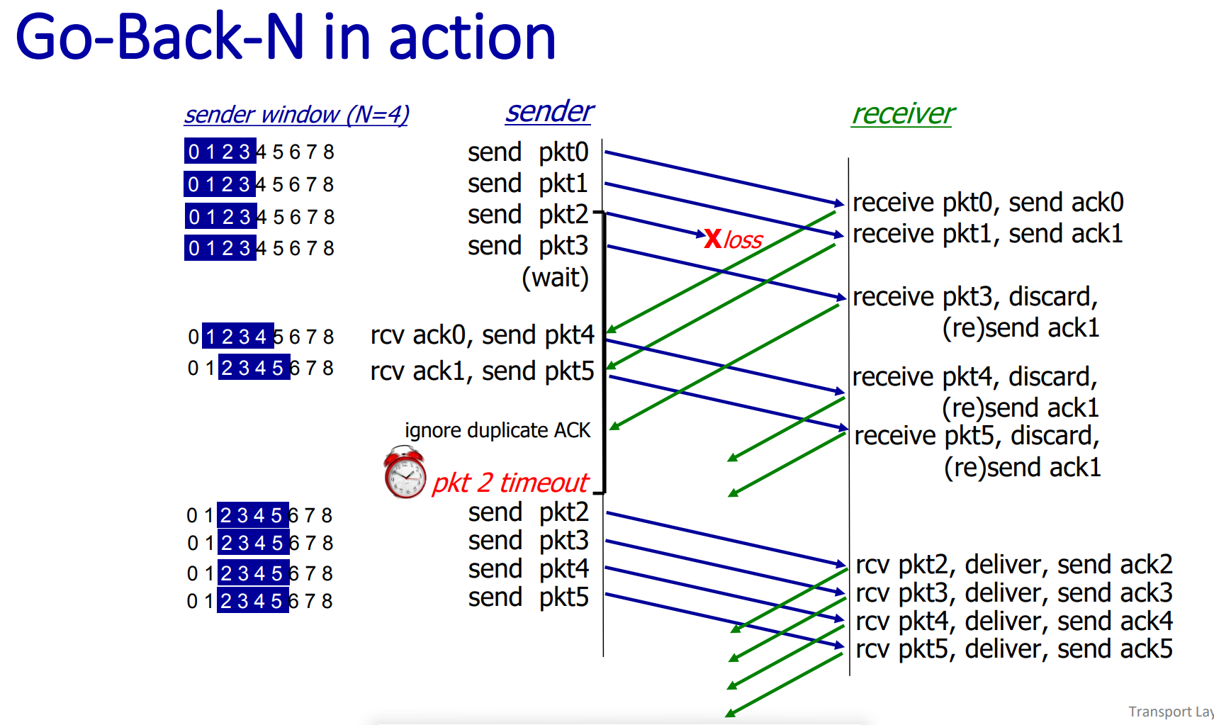
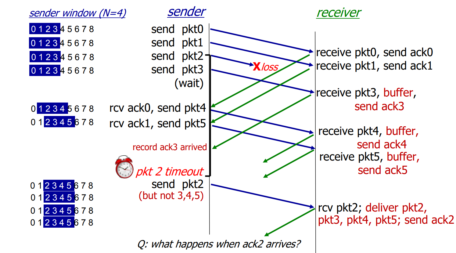
Go-Back-N: sender

sender: “window” of up to N, consecutive transmitted but unACKed pkts

cumulative ACK

timer for oldest in-flight packet

Selective repeat

receiver ****individually**** acknowledges all correctly received packets

sender times-out/retransmit individually for unACKed packets

Selective repeat : a dilemma

example :

seq #s : 0, 1, 2, 3

window size = 3

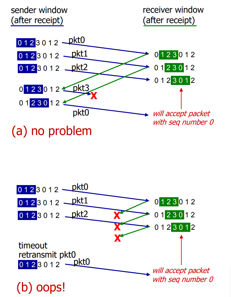
what relationship is neede between sequence # size and window size to avoid problem in scenario (b)?

→ 한정된 순서번호를 사용함. 즉, 한정된 순서번호의 허용치가 윈도우 사이즈 보다 크게 많지 않기 때문에 윈도우 사이즈보다 순서번호 허용치를 크게 늘리면 문제 해결됨

순서번호 허용치 값 ≥ 2 * 윈도우 크기

sequence number ≥ 2 * window size

TCP: overview

1. point-to-point : one sender, one receiver
2. reliable, in-order byte stream : no “message boundaries”
3. full duplex data : bi-directional data flow in same connection, MSS : maximum segment size
4. ****cumulative ACKs****
5. pipelining : TCp congestion and flow control set window size
6. ****connection-oriented :**** handshaking initialized sender, receiver state before data exchange
7. flow controlled : sender will not overwhelm receiver