이전까진 yolov4, yolov7을 사용해왔었는데 최근에 나온 yolov10을 사용해보려고 한다.
속도, 정확도면에서 이전 버전보다 높은 성능을 달성했다는데, 매우 기대중.
++ 12.09 자주 사용중인데, 사용하기도 편하고 성능도 좋고 아주 만족스럽다.
공식페이지에 설명이 잘되어있어서 따라하면 금방 적응된다. 여러 mode도 따로 정리되어있고, 영상도 있다.
아! 홈페이지에Ask AI라고 Ultralytics 전용 AI가 있는데 궁금한거 생길때마다 물어보면 대답도 잘해주고 관련 페이지도 캡션달아주고 해서 요긴하게 썼다.
환경설정
먼저 yolov10을 사용하기 위해 환경설정하고, 기본 모델을 테스트해보려고 한다.
이 게시글을 보고 따라했다.
지금 환경은
pytorch 2.2
python 3.10
cuda 12.3
yolov10을 설치하고, 필요한 패키지 설치하기
git clone https://github.com/THU-MIG/yolov10.git
cd yolov10
pip install -r requirements.txt
pip install -e .
HOME 위치를 설정해줬다.
난 yolov10이라는 폴더를 만들어서 관리할 것임으로 현재 위치에서 yolov10을 추가해준다.
import os
HOME = os.getcwd() + "/yolov10"
print(HOME)
pre-trained된 weights파일들을 다운로드해준다.
!mkdir -p {HOME}/weights
!wget -P {HOME}/weights -q https://github.com/THU-MIG/yolov10/releases/download/v1.1/yolov10n.pt
!wget -P {HOME}/weights -q https://github.com/THU-MIG/yolov10/releases/download/v1.1/yolov10s.pt
!wget -P {HOME}/weights -q https://github.com/THU-MIG/yolov10/releases/download/v1.1/yolov10m.pt
!wget -P {HOME}/weights -q https://github.com/THU-MIG/yolov10/releases/download/v1.1/yolov10b.pt
!wget -P {HOME}/weights -q https://github.com/THU-MIG/yolov10/releases/download/v1.1/yolov10x.pt
!wget -P {HOME}/weights -q https://github.com/THU-MIG/yolov10/releases/download/v1.1/yolov10l.pt
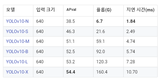
!ls -lh {HOME}/weights[출처] 참고로 모델 이름은 이런 뜻을 가지고있다.
- YOLOv10-N: 리소스가 극도로 제한된 환경을 위한 나노 버전입니다.
- YOLOv10-S: 속도와 정확성의 균형을 맞춘 소형 버전입니다.
- YOLOv10-M: 일반 용도의 중간 버전입니다.
- YOLOv10-B: 정확도를 높이기 위해 폭을 늘린 균형 잡힌 버전입니다.
- YOLOv10-L: 계산 리소스가 증가하지만 정확도가 더 높은 대형 버전입니다.
- YOLOv10-X: 정확도와 성능을 극대화하는 초대형 버전입니다.
이제 yolov10을 사용하기 위해 import를 시도하면,
from ultralytics import YOLOv10
에러가 난다!
⛔
attributeerror: module 'cv2.dnn' has no attribute 'dictvalue'
✅ opencv-python을 '4.8.0.74'로 다운그레이드해준다.
sudo pip install opencv-python==4.8.0.74
사진 한장 detect하고 결과 확인해보기.
from ultralytics import YOLOv10

model = YOLOv10(f'{HOME}/weights/yolov10n.pt')
results = model(source=f'{HOME}/bus.jpg', conf=0.25)
print(results[0].boxes.xyxy)
print(results[0].boxes.conf)
print(results[0].boxes.cls)
잘 나온다.
tensor([[6.8266e+00, 2.3275e+02, 8.0222e+02, 7.4057e+02],
[2.2210e+02, 4.0577e+02, 3.4420e+02, 8.6220e+02],
[4.8840e+01, 3.9576e+02, 2.4582e+02, 9.0808e+02],
[6.7007e+02, 3.9544e+02, 8.0969e+02, 8.7370e+02],
[2.7932e-01, 5.5142e+02, 6.0692e+01, 8.7015e+02]], device='cuda:0')
tensor([0.9502, 0.9022, 0.9010, 0.8932, 0.5015], device='cuda:0')
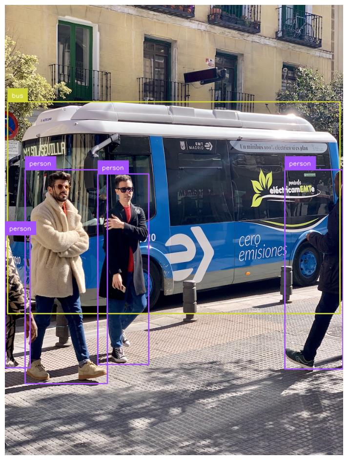
tensor([5., 0., 0., 0., 0.], device='cuda:0')결과를 시각화해서 볼껀데 supervision을 사용할꺼라 설치해주고,
sudo pip install supervision
코드를 실행한다.
import cv2
import supervision as sv
from ultralytics import YOLOv10

model = YOLOv10(f'{HOME}/weights/yolov10n.pt')
image = cv2.imread(f'{HOME}/bus.jpg')
results = model(image)[0]
detections = sv.Detections.from_ultralytics(results)

bounding_box_annotator = sv.BoundingBoxAnnotator()
label_annotator = sv.LabelAnnotator()

annotated_image = bounding_box_annotator.annotate(scene=image, detections=detections)
annotated_image = label_annotator.annotate(scene=annotated_image, detections=detections)

sv.plot_image(annotated_image)
이미지로 볼 수 있다.
custom data로 train하기
학습하기 위해선 내 dataset을 yolov10가 학습가능한 모양으로 만들어야한다.
yaml 파일에 내 데이터 경로, class 갯수와 이름을 입력한다.
train: /content/my_dataset/images/train
val: /content/my_dataset/images/val

nc: N     # N for number of classes
names: ['class1', 'class2', ..., 'classN']
++ 모든 파일의 경로를 적어둔 txt파일을 넣어도 된다.
train: /home/work/my_dataset/train.txt
val: /home/work/my_dataset/val.txt
test: /home/work/my_dataset/test.txt
image, label 파일 tree는 아래와 같다.
/my_dataset
  /train
    /images
      image1.jpg
      image2.jpg
      ...
    /labels
      image1.txt
      image2.txt
      ...
  /val
    /images
      image1.jpg
      image2.jpg
      ...
    /labels
      image1.txt
      image2.txt
  /test
    /images
      image1.jpg
      image2.jpg
      ...
    /labels
      image1.txt
      image2.txt
      ...
  data.yaml
yaml파일을 보면 train, val, test의 이미지가 들어있는 폴더가 적혀있다.
이 images폴더에 학습에 사용될 이미지가 들어있고, 같은 위치 labels폴더에 이미지랑 같은 이름의 txt파일이 들어있어야한다.
txt파일에서 좌표값은 0에서 1사이로 정규화 되어있다.
class_id center_x center_y width height
여기 적혀있는것처럼 하나의 이미지에 들어있는 모든 객체를 다 적어주면 된다.
(보통 4~6번째자리에서 끊어준다.)
1 0.617 0.3594420600858369 0.114 0.17381974248927037
1 0.094 0.38626609442060084 0.156 0.23605150214592274
1 0.295 0.3959227467811159 0.13 0.19527896995708155
1 0.785 0.398068669527897 0.07 0.14377682403433475
1 0.886 0.40879828326180256 0.124 0.18240343347639484
1 0.723 0.398068669527897 0.102 0.1609442060085837
2 0.541 0.35085836909871243 0.094 0.16952789699570817
2 0.428 0.4334763948497854 0.068 0.1072961373390558
3 0.375 0.40236051502145925 0.054 0.1351931330472103
3 0.976 0.3927038626609442 0.044 0.17167381974248927
데이터를 준비했다면 학습명령어를 입력한다.
yolo task=detect mode=train epochs=25 batch=32 plots=True model='/content/weights/yolov10n.pt' data='/content/X-Ray-Baggage-3/data.yaml'
난 GPU도 여러개 사용하고 싶고 저장 위치로 바꾸고 싶어서 매개변수를 몇개 추가했다.
yolo task=detect mode=train epochs=300 batch=16 plots=True model='weights/yolov10m.pt' data='../data/data.yaml' imgsz=640 device=0,1,2,3 project='my_data' name='m_b16_e300'
여기서 optimizer를 바꾼다던가 dropout 넣기 등등 알아서 튜닝하면 된다.
매개변수 설명은 여기 Train Settings에서 확인 가능하다.
학습이 진행중인데 labels폴더를 확인하는 와중에 이런 경고가 뜬다.
train: WARNING ⚠️ /home/work/object-detection/data/train/images/ND166001_025_00005395.jpg: 1 duplicate labels removed
train: WARNING ⚠️ /home/work/object-detection/data/train/images/ND166002_001_00003957.jpg: 1 duplicate labels removed
train: WARNING ⚠️ /home/work/object-detection/data/train/images/ND166002_010_00000360.jpg: 1 duplicate labels removed
train: WARNING ⚠️ /home/work/object-detection/data/train/images/NG159003_002_00007435.jpg: 1 duplicate labels removed검색해보니 labels.txt 파일에 중복된 행이 있다는 경고였다.
해당 파일을 확인해보니 똑같은 object가 두개 적혀있다.
전체 data를 돌면서 중복된 행을 제거해줬다.
train한 weight로 inference하기
학습이 끝나면 아까 설정한 my_data/m_b16_e300 폴더 안에 결과가 저장된다.
weights 폴더에 best.pt와 last.pt가 저장되는데 best.pt을 꺼내서 추론에 사용해봤다.
from ultralytics import YOLOv10

model_path = '/yolov10/my_data/m_e300/weights/best.pt'
model = YOLOv10(model_path)
image_path = 'test_image_path.jpg'
results = model(source=image_path, conf=0.25)

print(results[0].boxes.xyxy)
print(results[0].boxes.conf)
print(results[0].boxes.cls)
추론시간도 알려주고,
boxes를 print하면 tensor로 나온다.
image 1/1 test_image_path.jpg: 384x640 2 white-smokes, 1 chimney-smoke, 16.7ms
Speed: 2.1ms preprocess, 16.7ms inference, 1.1ms postprocess per image at shape (1, 3, 384, 640)
tensor([[1135.2274,   93.0486, 1312.5896,  255.6580],
        [1036.3219,  215.8592, 1074.8546,  255.1565],
        [1096.3506,  224.6951, 1144.8625,  251.6425]], device='cuda:0')
tensor([0.8986, 0.7767, 0.7041], device='cuda:0')
tensor([1., 5., 1.], device='cuda:0')
전체 results[0].boxes를 보면 box도 xyxy, xywh 등 원하는 모양 꺼내서 쓸 수 있고, tracker로 추론하면 box의 id도 추적해준다.
(영상 검출할때 tracker 유용하게 잘썼어요👍)
cls: tensor([5., 1., 5., 1., 1.], device='cuda:0')
conf: tensor([0.8780, 0.8104, 0.7732, 0.4608, 0.2961], device='cuda:0')
data: tensor([[1.2147e+03, 1.2917e+02, 1.3588e+03, 2.9973e+02, 8.7798e-01, 5.0000e+00],
        [1.3539e+03, 2.6210e+02, 1.4101e+03, 2.9861e+02, 8.1038e-01, 1.0000e+00],
        [1.1141e+03, 2.3128e+02, 1.1678e+03, 2.8862e+02, 7.7325e-01, 5.0000e+00],
        [1.1838e+03, 2.5435e+02, 1.2365e+03, 2.9039e+02, 4.6075e-01, 1.0000e+00],
        [1.2409e+03, 2.6693e+02, 1.2642e+03, 2.9610e+02, 2.9607e-01, 1.0000e+00]], device='cuda:0')
id: None
is_track: False
orig_shape: (1080, 1920)
shape: torch.Size([5, 6])
xywh: tensor([[1286.7875,  214.4473,  144.1223,  170.5587],
        [1381.9915,  280.3526,   56.1826,   36.5143],
        [1140.9518,  259.9515,   53.7097,   57.3403],
        [1210.1781,  272.3670,   52.6726,   36.0438],
        [1252.5396,  281.5149,   23.2715,   29.1737]], device='cuda:0')
xywhn: tensor([[0.6702, 0.1986, 0.0751, 0.1579],
        [0.7198, 0.2596, 0.0293, 0.0338],
        [0.5942, 0.2407, 0.0280, 0.0531],
        [0.6303, 0.2522, 0.0274, 0.0334],
        [0.6524, 0.2607, 0.0121, 0.0270]], device='cuda:0')
xyxy: tensor([[1214.7263,  129.1679, 1358.8486,  299.7266],
        [1353.9001,  262.0954, 1410.0828,  298.6098],
        [1114.0969,  231.2813, 1167.8066,  288.6216],
        [1183.8418,  254.3451, 1236.5144,  290.3889],
        [1240.9038,  266.9280, 1264.1753,  296.1018]], device='cuda:0')
xyxyn: tensor([[0.6327, 0.1196, 0.7077, 0.2775],
        [0.7052, 0.2427, 0.7344, 0.2765],
        [0.5803, 0.2141, 0.6082, 0.2672],
        [0.6166, 0.2355, 0.6440, 0.2689],
        [0.6463, 0.2472, 0.6584, 0.2742]], device='cuda:0')
result[0].show() 하면 바로 결과 이미지창 띄워준다.
아까 yolov10 기본 모델 사용할 때랑 똑같이 시각화해봤다.
import supervision as sv

results = model(image)[0]
detections = sv.Detections.from_ultralytics(results)

bounding_box_annotator = sv.BoundingBoxAnnotator()
label_annotator = sv.LabelAnnotator()

annotated_image = bounding_box_annotator.annotate(
    scene=image, detections=detections)
annotated_image = label_annotator.annotate(
    scene=annotated_image, detections=detections)

sv.plot_image(annotated_image)
이렇게 class마다 색도 다르게 해서 나옴
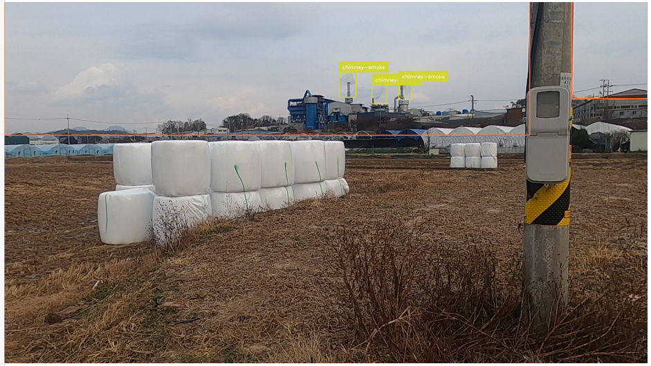
ultralytics는 처음 사용해봤는데 편하고 좋네.
++ 그냥 편한정도가 아니다. 최고에요 ultralytics 사랑해요 ultralytics