Setting
데이터를 좀 더 알기 쉽게 표현할 수 있도록 만들어 준다. 다음과 같은 코드로 세팅이 완료된다.
import pandas as pd
pd.plotting.register_matplotlib_converters()
import matplotlib.pyplot as plt
%matplotlib inline
import seaborn as sns
%matplotlib inline은 notebook을 실행한 브라우저에서 바로 그림을 볼 수 있도록 해주는 것이다.
pandas로 데이터를 열어주고 그래프로 표현하는 것들은 matplotlib.pyplot(plt), seaborn을 이용한다.
pd.plotting.register_matplotlib_converters()은 객체에 matplotlib를 그려내기 위한 변환기 이다.(그냥 등록한다고 알아두자.)
어떤 데이터에 어떤 plot을 이용할 것인가?
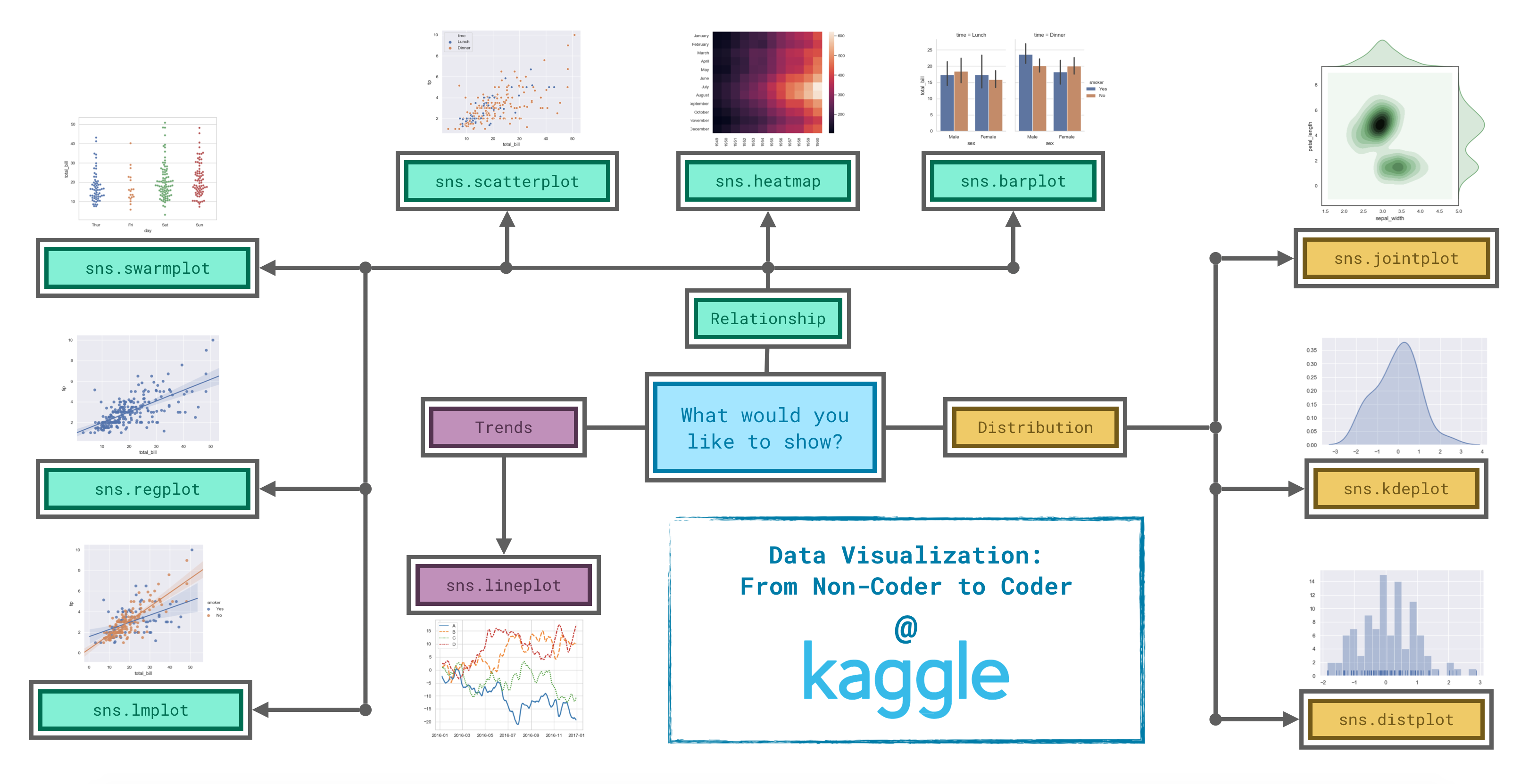
굉장히 다양한 plot 이 있는데, 위 그림처엄 나눌 수 있다고 한다.
Trend
sns.lineplot
# Line chart showing daily global streams of 'Shape of You'
sns.lineplot(data=spotify_data['Shape of You'], label="Shape of You")

# Line chart showing daily global streams of 'Despacito'
sns.lineplot(data=spotify_data['Despacito'], label="Despacito")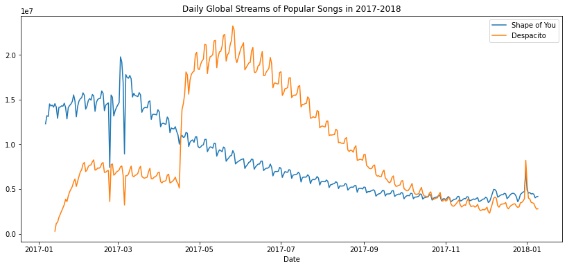
이런 식으로 시간에 따른 Stream 수 를 표현할 수도 있게 된다.
그래서 lineplot은 Trend를 알아볼 때 이용하게 된다.
Relationship
sns.barplot
sns.barplot(x=flight_data.index, y=flight_data['NK'])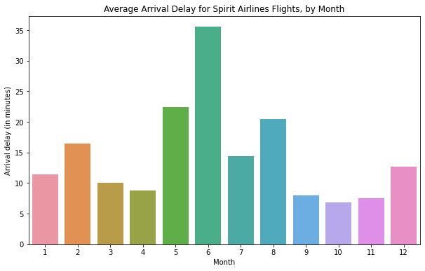
비슷한 것으로 countplot이 있다 이용방법은 같으나, countplot은 개수를 셀 데이터의 정보만 x축에 대입하면 된다.
sns.heatmap
sns.heatmap(data=flight_data, annot=True)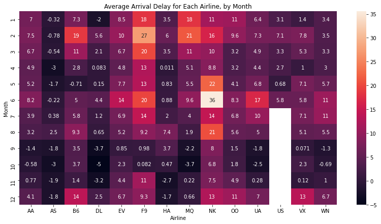
annot=True는 heatmap에 숫자를 표기하기 위해서 이다. heatmap 또한 데이터간의 관계를 표현하기 위해 많이 쓰이게 되는데, 가장 큰 수나 가장 작은 수를 찾거나 할 때 쉽게 찾을 수 있다는 장점이 있다.
sns.scatterplot
sns.scatterplot
sns.scatterplot(x=insurance_data['bmi'], y=insurance_data['charges'])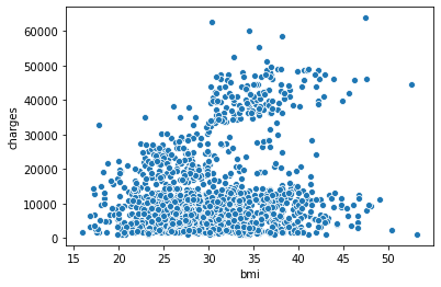
x, y의 데이터가 모두 int 형이여야 그래프를 만들 수 있다는 특징이 있다. x='bmi' , y='charges', data=insurance_data로 해도 가능하다.
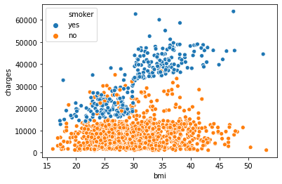
데이터 중 int형 type만 두게 만드려면 다음과 같은 코드를 이용하면 된다.
# To keep things simple, we'll use only numerical predictors
X = X_full.select_dtypes(exclude=['object'])
X_test = X_test_full.select_dtypes(exclude=['object'])
여기에서 hue=insurance_data['smoker']라는 데이터를 추가하게 되면, 추가적인 데이터까지 구분이 가능하다.
sns.regplot
sns.regplot(x=insurance_data['bmi'], y=insurance_data['charges'])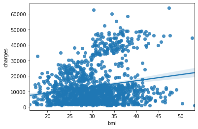
위의 scatterplot에서 방향성을 가지도록 선을 하나 그은 것이다.
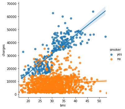
이 또한 hue="smoker"를 추가하면 색깔별로 서로 다른 regressor 선을 만들 수 있다.
sns.swarmplot
sns.swarmplot(x=insurance_data['smoker'],
              y=insurance_data['charges'])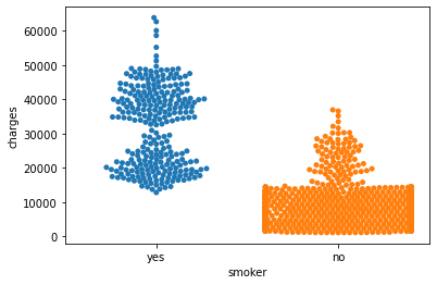
이거는 이용해보려 했는데, 형태에 관련된 에러가 계속 되고 실행이 잘 안되서 string 형태의 데이터를 encoding 하는 방법을 써보기로 하였다.
Distribution
어떤 식으로 데이터가 분리되었는지 알 수 있게 하기 위해 아래와 같은 방법을 이용한다.
sns.distplot
Histogram과 같다.
sns.distplot(a=iris_data['Petal Length (cm)'], kde=False)
kde=False는 histogram에 선을 긋지 않게 하기 위해서 이다. 만약 저것을 없앤다면 아래와 같이 선이 그려질 것이다.
이 distplot의 특징은 a를 column의 변수로 이용한다는 점이다.
sns.kdeplot
sns.kdeplot(data=iris_data['Petal Length (cm)'], shade=True)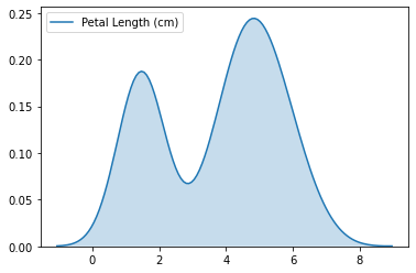
이를 2D로 만들고 싶다면?
# 2D KDE plot
sns.jointplot(x=iris_data['Petal Length (cm)'], y=iris_data['Sepal Width (cm)'], kind="kde")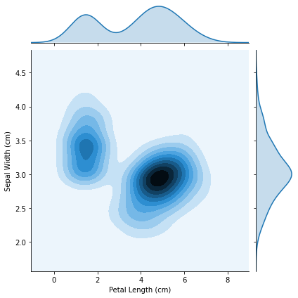
이들 또한 하나의 data feature 만 넣을 수 있다는 점에 주의하자. shade는 부드럽게 만들어준다.
Tips
만약 여러 개의 feature들을 구별하고 싶다면 다음과 같은 방법을 이용하자.
# Histograms for each species
sns.distplot(a=iris_set_data['Petal Length (cm)'], label="Iris-setosa", kde=False)
sns.distplot(a=iris_ver_data['Petal Length (cm)'], label="Iris-versicolor", kde=False)
sns.distplot(a=iris_vir_data['Petal Length (cm)'], label="Iris-virginica", kde=False)

# Add title
plt.title("Histogram of Petal Lengths, by Species")

# Force legend to appear
plt.legend()
색깔 setting
plt.figure(figsize=(,)) #원하는 figsize 넣기
sns.set(style="darkgrid, dark, whitegrid, white, ticks) # 5개 중에서 선택