PyTorch 로지스틱 회귀

• 자료출처 : PyTorch로 시작하는 딥 러닝 입문

로지스틱 회귀

1. 이진 분류 (Binary Classification)

• 두 개의 선택지 중 정답을 고르는 경우(정답, 오답 / 합격, 불합격)에 활용하는게 이진분류
• 이진 분류를 풀기 위한 대표적인 알고리즘이 로지스틱 회귀(Logistic Regression)
• 두 개의 선택지를 가진 데이터의 분포는 S 형태의 그래프를 가진다.

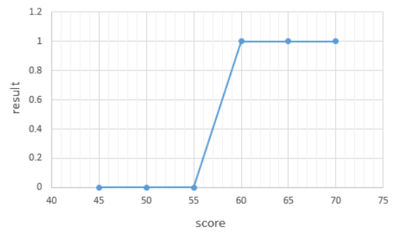
• S 그래프를 만들기 위해 선형회귀함수에 특정 함수 f 를 추가하는데 특정 함수 f 를 시그모이드 함수라고 함

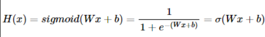
2. 시그모이드 함수

%matplotlib inline
import numpy as np 
import matplotlib.pyplot as plt # 맷플롯립 (시각화 도구)

def sigmoid(x): # 시그모이드 함수 정의
    return 1/(1+np.exp(-x))

# W 값을 변화시키면서 그래프 확인
x = np.arange(-5.0, 5.0, 0.1)
y1 = sigmoid(0.5*x)
y2 = sigmoid(x)
y3 = sigmoid(2*x)

plt.plot(x, y1, 'r', linestyle='--') # W의 값이 0.5일때
plt.plot(x, y2, 'g') # W의 값이 1일때
plt.plot(x, y3, 'b', linestyle='--') # W의 값이 2일때
plt.plot([0,0],[1.0,0.0], ':') # 가운데 점선 추가
plt.title('Sigmoid Function')
plt.show()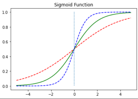

3. 비용함수 (Cost Function)

• 최적의 W와 b를 찾을 수 있는 비용함수를 정의
• 시그모이드 함수가 적용된 비용함수를 미분하면 선형회귀 때와는 다르게 아래와 같은 그래프가 나온다

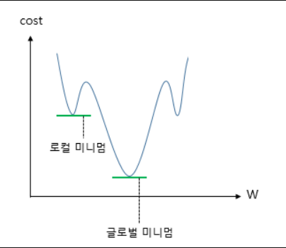
• 로컬 미니멈에 그치지 않고 글로벌 미니멈을 찾기 위해서 시그모이드 함수의 특징을 활용해야 한다.
• 시그모이드 함수의 출력값이 0과 1사이므로 y= 0.5인 로그함수를 충족한다.

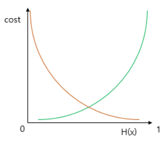
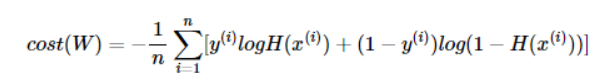
• 로그함수를 적용하면 아래와 같은 식이 나온다

4. 파이토치로 로지스틱 회귀 구현하기

import torch
import torch.nn as nn
import torch.nn.functional as F
import torch.optim as optim

torch.manual_seed(1)

<torch._C.Generator at 0x20ae0f61190>

# 텐서로 데이터 선언
x_data = [[1, 2], [2, 3], [3, 1], [4, 3], [5, 3], [6, 2]]
y_data = [[0], [0], [0], [1], [1], [1]]
x_train = torch.FloatTensor(x_data)
y_train = torch.FloatTensor(y_data)

print(x_train.shape)
print(y_train.shape)

torch.Size([6, 2])
torch.Size([6, 1])

W = torch.zeros((2, 1), requires_grad=True) # 크기는 2 x 1
b = torch.zeros(1, requires_grad=True)

# 로지스틱 회귀 가설식 수립 (시그모이드 활용하면 좀 더 쉽게 수립)
hypothesis = 1 / (1 + torch.exp(-(x_train.matmul(W) + b)))
# hypothesis = torch.sigmoid(x_train.matmul(W) + b)

print(hypothesis) # 예측값인 H(x) 출력

tensor([[0.5000],
        [0.5000],
        [0.5000],
        [0.5000],
        [0.5000],
        [0.5000]], grad_fn=<MulBackward0>)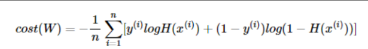

# 비용함수 구현 (오차 구하기)
losses = -(y_train * torch.log(hypothesis) + 
           (1 - y_train) * torch.log(1 - hypothesis))
print(losses)

tensor([[0.6931],
        [0.6931],
        [0.6931],
        [0.6931],
        [0.6931],
        [0.6931]], grad_fn=<NegBackward0>)

cost = losses.mean()
print(cost) # 오차결과 

tensor(0.6931, grad_fn=<MeanBackward0>)

5. 내장된 로지스틱회귀 함수활용

F.binary_cross_entropy(hypothesis, y_train)

tensor(0.6931, grad_fn=<BinaryCrossEntropyBackward0>)

x_data = [[1, 2], [2, 3], [3, 1], [4, 3], [5, 3], [6, 2]]
y_data = [[0], [0], [0], [1], [1], [1]]
x_train = torch.FloatTensor(x_data)
y_train = torch.FloatTensor(y_data)

# 전체 코드 정리 

# 모델 초기화
W = torch.zeros((2, 1), requires_grad=True)
b = torch.zeros(1, requires_grad=True)
# optimizer 설정
optimizer = optim.SGD([W, b], lr=1)

nb_epochs = 1000
for epoch in range(nb_epochs + 1):

    # Cost 계산
    hypothesis = torch.sigmoid(x_train.matmul(W) + b)
    cost = -(y_train * torch.log(hypothesis) + 
             (1 - y_train) * torch.log(1 - hypothesis)).mean()

    # cost로 H(x) 개선
    optimizer.zero_grad()
    cost.backward()
    optimizer.step()

    # 100번마다 로그 출력
    if epoch % 100 == 0:
        print('Epoch {:4d}/{} Cost: {:.6f}'.format(
            epoch, nb_epochs, cost.item()
        ))

Epoch    0/1000 Cost: 0.693147
Epoch  100/1000 Cost: 0.134722
Epoch  200/1000 Cost: 0.080643
Epoch  300/1000 Cost: 0.057900
Epoch  400/1000 Cost: 0.045300
Epoch  500/1000 Cost: 0.037261
Epoch  600/1000 Cost: 0.031673
Epoch  700/1000 Cost: 0.027556
Epoch  800/1000 Cost: 0.024394
Epoch  900/1000 Cost: 0.021888
Epoch 1000/1000 Cost: 0.019852

# 현재 W와 b로 결과 예측
hypothesis = torch.sigmoid(x_train.matmul(W) + b)
print(hypothesis)

tensor([[2.7648e-04],
        [3.1608e-02],
        [3.8977e-02],
        [9.5622e-01],
        [9.9823e-01],
        [9.9969e-01]], grad_fn=<SigmoidBackward0>)

# 0.5를 기준으로 True 와 False 나누기
prediction = hypothesis >= torch.FloatTensor([0.5])
print(prediction)

tensor([[False],
        [False],
        [False],
        [ True],
        [ True],
        [ True]])

# 훈련 후 W 와 b 출력
print(W)
print(b)

tensor([[3.2530],
        [1.5179]], requires_grad=True)
tensor([-14.4819], requires_grad=True)