순환신경망 RNN

• 자료출처 : PyTorch로 시작하는 딥 러닝 입문
• RNN은 가장 기본적인 시퀀스(Sequence) 모델이다.
• 시퀀스 모델은 입력과 출력을 시퀀스 단위로 처리하는 모델을 말한다. 예를 들어 단어 시퀀스는 문장을 의미한다.

1. RNN (Recurrent Neural Network) 개념

• 앞서 배운 신경망들은 전부 은닉층에서 활성화 함수를 지나서 출력층 방향으로 향하는 피드 포워드 신경망(Feed Forward Neural Network)다.
• 반면 RNN은 은닉층의 노드에 활성화 함수 결과값을 출력층 방향으로도 보내고, 한번 더 계산해서 입력 값으로 보내는 특징을 가지고 있다.
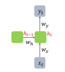
• x는 입력 벡터, y는 출력 벡터다. RNN의 은닉층에서 활성화 함수 결과를 내보내는 역할을 하는 노드를 셀(Cell)이라고 한다.

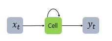
• 이 셀은 이전의 값을 기억하려고 하는 일종의 메모리 역할을 수행하므로 이를 메모리 셀 또는 RNN 셀이라고 표현한다.
• 은닉층의 메모리 셀은 각각의 시점(time step)의 바로 이전 시점에 나온 값을 자신의 입력으로 사용하는 재귀적 활동을 함.
• 현재 시점(t)의 메모리 셀이 갖는 값은 과거 메모리 셀들의 값에 영향을 받음
• 메모리 셀이 출력층 방향으로 또는 다음 시점(t+1)의 자신에게 보내는 값을 은닉 상태(hidden state)라고 한다.
• 정리하면 t 시점의 메모리 셀은 t-1 시점의 메모리 셀이 보낸 은닉 상태값을 t 시점의 은닉 상태 계산을 위한 값으로 사용한다.
  
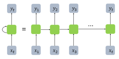
• RNN을 위 그림처럼 표현할 수 있는데 좌측처럼 화살표로 사이클을 그려 재귀적으로 표현할 수도 있지만, 우측처럼 여러시점으로 펼쳐서 표현하기도 한다. 둘 다 같은 RNN을 표현하고 있다.
• 피드 포워드 신경망에선 뉴런이라는 단위를 사용했지만, RNN에선 뉴런이란 단위보단 벡터, 은닉층보단 은닉상태라는 표현을 자주 사용한다. 둘의 차이를 비교하기 위해 RNN을 뉴런 단위로 시각화 했다.
  
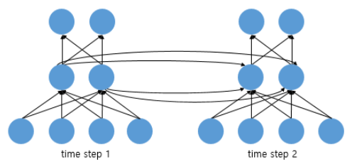
• 입력 벡터 차원 4, 은닉상태 크기 2, 출력 벡터 차원 2인 RNN의 그림이다.
• 뉴런 단위로 보면, 입력층 뉴런 4, 은닉층 뉴런 2, 출력층 뉴런 2 가 된다.

2. RNN의 활용

• RNN은 입력과 출력의 길이를 다르게 설계할 수 있다. 일대다, 다대일, 다대다 형태로 활용되며 다양한 용도로 활용된다.
  
• 일대다 모델의 경우 하나의 이미지에 대해 다양한 사진의 제목을 출력하는 이미지 캡셔닝 (Image Captioning) 작업에 사용할 수 있다. 사진 제목은 단어들의 나열이므로 시퀀스 출력이다.
  
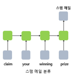
• 다대일 모델은 리뷰 등 텍스트의 긍정,부정을 판별하는 감성분류(sentiment classification)나 스팸 메일 분류(spam detection)에 사용할 수 있다.
  
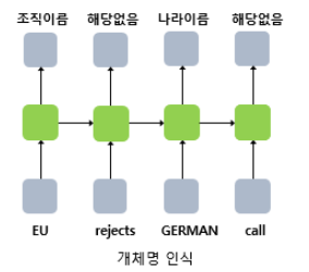
• 다대다 모델은 입력 문장으로 부터 대답 문장을 출력하는 챗봇과 입력 문장을 번역하는 번역기, 개체명 인식이나 품사 태깅과 같은 작업에 사용된다.

3. RNN 수식 정의

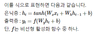
• 현재 시점(t)의 은닉 상태값은 ht라고>정의한다. ht 값의 계산을 위해 입력층의 가중치와 이전 시점(t-1)의 가중치, 총 두 개의 가중치를 갖제 된다.
  
  
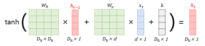
• 단어 벡터의 차원(d), 은닉 상태의 크기(Dh)는 모두 4, 배치 크기를 1로 가정한 RNN 은닉층 연산은 그림과 같다.
  

4. 파이썬 구현

import numpy as np

timesteps = 10 # 시점의 수. NLP에서는 보통 문장의 길이가 된다.
input_size = 4 # 입력의 차원. NLP에서는 보통 단어 벡터의 차원이 된다.
hidden_size = 8 # 은닉 상태의 크기. 메모리 셀의 용량이다.

inputs = np.random.random((timesteps, input_size)) # 입력에 해당되는 2D 텐서
# 쉬운 이해를 위해 2D 텐서로 가정했으나 실제 파이토치에선 batch_size가 포함된 3D 텐서의 입력을 받는다.

hidden_state_t = np.zeros((hidden_size,)) # 초기 은닉 상태는 0(벡터)로 초기화
# 은닉 상태의 크기 hidden_size로 은닉 상태를 만듬.

print(hidden_state_t) # 8의 크기를 가지는 은닉 상태. 현재는 초기 은닉 상태로 모든 차원이 0의 값을 가짐.

[0. 0. 0. 0. 0. 0. 0. 0.]

# 가중치와 편향 정의
Wx = np.random.random((hidden_size, input_size))  # (8, 4)크기의 2D 텐서 생성. 입력에 대한 가중치.
Wh = np.random.random((hidden_size, hidden_size)) # (8, 8)크기의 2D 텐서 생성. 은닉 상태에 대한 가중치.
b = np.random.random((hidden_size,)) # (8,)크기의 1D 텐서 생성. 이 값은 편향(bias).

print(np.shape(Wx))
print(np.shape(Wh))
print(np.shape(b))

(8, 4)
(8, 8)
(8,)

# RNN 층 동작
total_hidden_states = []

# 메모리 셀 동작
for input_t in inputs: # 각 시점에 따라서 입력값이 입력됨.
  output_t = np.tanh(np.dot(Wx,input_t) + np.dot(Wh,hidden_state_t) + b) # Wx * Xt + Wh * Ht-1 + b(bias)
  total_hidden_states.append(list(output_t)) # 각 시점의 은닉 상태의 값을 계속해서 축적
  print(np.shape(total_hidden_states)) # 각 시점 t별 메모리 셀의 출력의 크기는 (timestep, output_dim)
  hidden_state_t = output_t

total_hidden_states = np.stack(total_hidden_states, axis = 0) 
# 출력 시 값을 깔끔하게 해준다.

print(total_hidden_states) # (timesteps, output_dim)의 크기. 이 경우 (10, 8)의 크기를 가지는 메모리 셀의 2D 텐서를 출력.

(1, 8)
(2, 8)
(3, 8)
(4, 8)
(5, 8)
(6, 8)
(7, 8)
(8, 8)
(9, 8)
(10, 8)
[[0.99994788 0.9999617  0.99995532 0.99993631 0.99992509 0.99997685
  0.9999986  0.9999828 ]
 [0.99973439 0.99991707 0.99985339 0.99985522 0.99985771 0.99992208
  0.99999709 0.99996431]
 [0.99977628 0.99995234 0.99975985 0.99988085 0.99989981 0.99997422
  0.99999853 0.99997849]
 [0.99975057 0.99995433 0.99989045 0.99975765 0.99991362 0.99989079
  0.99999599 0.99995614]
 [0.99997016 0.99996681 0.999964   0.99997593 0.99995089 0.99999126
  0.99999949 0.99999236]
 [0.99970514 0.99994434 0.9997721  0.99988929 0.99991427 0.99996127
  0.99999855 0.99997848]
 [0.99982007 0.99989741 0.99990778 0.99991067 0.99985279 0.99992823
  0.99999761 0.9999706 ]
 [0.99982146 0.99989636 0.99990522 0.99989431 0.99982903 0.99992443
  0.99999712 0.99996608]
 [0.99985846 0.99990951 0.99991321 0.99989168 0.99982538 0.99993841
  0.99999708 0.99996645]
 [0.99980879 0.99993696 0.99982009 0.9998787  0.99986009 0.99996607
  0.99999799 0.99997338]]

5. 파이토치의 nn.RNN()

import torch
import torch.nn as nn

input_size = 5 # 입력의 크기
hidden_size = 8 # 은닉 상태의 크기

# (batch_size, time_steps, input_size)
inputs = torch.Tensor(1, 10, 5) # 배치크기 x 시점의 수 x 매 시점 둘어가는 입력

# RNN 셀 만들기
cell = nn.RNN(input_size, hidden_size, batch_first=True)

# 입력 텐서를 RNN 셀에 입력
outputs, _status = cell(inputs)

print(outputs.shape) # 모든 time-step의 hidden_state

torch.Size([1, 10, 8])

print(_status.shape) # 최종 time-step의 hidden_state

torch.Size([1, 1, 8])

• 모든 시점의 은틱상태는 (1,10,8), 마지막 시점의 은닉상태는 (1,1,8)의 크기를 가진다.

6. 깊은 순환신경망과 양방향 순환신경망

깊은 순환신경망

• RNN도 다수의 은닉층을 가지며 깊은 순환 신경망을 가질 수 있다.
• 깊은 순환신경망을 파이토치로 구현할 땐 nn.RNN()의 인자인 num_layers에 값을 전달하여 층을 쌓는다.
• 층이 2개인 깊은 순환신경망의 경우, 앞서 실습했던 임의의 입력에 대해 출력이 달라진다.

# (batch_size, time_steps, input_size)
inputs = torch.Tensor(1, 10, 5)

# num_layer = 2 (은닉층이 2개)
cell = nn.RNN(input_size = 5, hidden_size = 8, num_layers = 2, batch_first=True)

print(outputs.shape) # 모든 time-step의 hidden_state

torch.Size([1, 10, 8])

print(_status.shape) # (층의 개수, 배치 크기, 은닉 상태의 크기)

torch.Size([2, 1, 8])

양방향 순환신경망

• 아래 괄호를 채우기 위해선, 앞의 내용 뿐만 아니라 뒤의 내용도 알아야 한다.
  - Exercise is very effective a [ ] belly fat.

• 이처럼 이전 시점 뿐만 아니라 이후 시점의 데이터도 활용하기 위해 고안된 것이 양방향 RNN 이다.
  

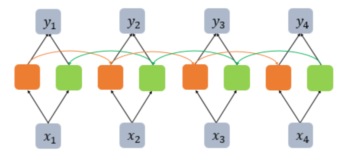
• 양방향 RNN은 하나의 출력값을 예측하기 위해 기본적으로 두 개의 메모리 셀을 사용한다.

• 첫 번째 메모리 셀은 앞 시점의 은닉상태(Forward State)를 전달받아 현재의 은닉상태를 계산한다.

• 두 번째 메모리 셀은 뒤 시점의 은닉상태(Backward State)를 전달받아 현재의 은닉상태를 계산한다

• 위의 그림에서 주황색은 Forward State를 초록색 메모리 셀은 Backward State에 해당된다.

깊은 양방향 순환신경망

• 양방향 RNN도 다수의 은닉층을 가질 수 있다.

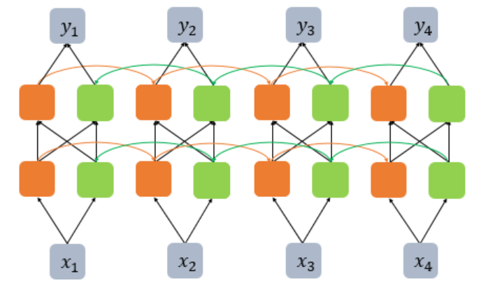
• 다른 인공신경망 모델도 마찬가지지만 은닉층을 무조건 추가한다고 모델의 성능이 좋아지는 것은 아니다.
• 은닉층을 추가하면 학습할 수 있는 양이 많아지지만 그만큼 훈련 데이터도 많이 필요하다.

깊은 양방햔 순환신경망 파이썬 구현

# (batch_size, time_steps, input_size)
inputs = torch.Tensor(1, 10, 5)

cell = nn.RNN(input_size = 5, hidden_size = 8, num_layers = 2, batch_first=True, bidirectional = True)

outputs, _status = cell(inputs)

print(outputs.shape) # (배치 크기, 시퀀스 길이, 은닉 상태의 크기 x 2)

torch.Size([1, 10, 16])

print(_status.shape) # (층의 개수 x 2, 배치 크기, 은닉 상태의 크기)

torch.Size([4, 1, 8])