회귀(1) - 선형회귀 : 보스턴 주택가격 예측

이 글은 파이썬 머신러닝 완벽 가이드 책 내용을 기반으로 정리했습니다.
내용출처 : 파이썬 머신러닝 완벽가이드

• 데이터 값이 평균으로 돌아가려는 경향을 이용한 통계학 기법이다. 가장 많이 쓰이는 건 선형 회귀 모델이다.
• 실제 값과 예측값의 차이를 최소화하는 직선형 회귀선을 최적화하는 방식으로 규제 종류에 따라 릿지, 라쏘, 엘라스틱넷, 로지스틱 회귀로 나뉜다.
• 우선 규제가 적용되지 않는 단순 선형회귀를 구현해본다.

사이킷런 선형회귀를 이용한 보스턴 주택가격 예측

• 사이킷런 linear_models 모듈은 매우 다양한 종류이 선형 기반 회귀를 클래스로 구현해 제공한다.

import numpy as np
import matplotlib.pyplot as plt
import pandas as pd
import seaborn as sns
from scipy import stats  # 과학용 계산 라이브러리
from sklearn.datasets import load_boston  # 사이킷런 데이타셋
%matplotlib inline
import warnings
warnings.filterwarnings('ignore') # 경고무시

데이터 로드 및 확인

# boston 데이타셋 로드 
boston = load_boston()

# boston 데이타셋 DataFrame 변환
df = pd.DataFrame(boston.data, columns = boston.feature_names)

# target array로 주택가격(price)을 추가함.
df['PRICE'] = boston.target
print('Boston 데이타셋 크기 :', df.shape)
df.head(2)

Boston 데이타셋 크기 : (506, 14)

• CRIM: 지역별 범죄 발생률
• ZN: 25,000평방피트를 초과하는 거주 지역의 비율
• NDUS: 비상업 지역 넓이 비율
• CHAS: 찰스강에 대한 더미 변수(강의 경계에 위치한 경우는 1, 아니면 0)
• NOX: 일산화질소 농도
• RM: 거주할 수 있는 방 개수
• AGE: 1940년 이전에 건축된 소유 주택의 비율
• DIS: 5개 주요 고용센터까지의 가중 거리
• RAD: 고속도로 접근 용이도
• TAX: 10,000달러당 재산세율
• PTRATIO: 지역의 교사와 학생 수 비율
• B: 지역의 흑인 거주 비율
• LSTAT: 하위 계층의 비율
• PRICE: 본인 소유의 주택 가격(중앙값) - 종속변수 (위의 건 독립변수)

# 2x4 subplot 이용. axs는 4x2 
fig, axs = plt.subplots(figsize=(16,8), ncols=4, nrows=2)

lm_features = ['RM','ZN','INDUS','NOX','AGE','PTRATIO','LSTAT','RAD']

# i에는 인덱스가 feature에는 RM ~ RAD까지 순차적으로 들어감
for i, feature in enumerate(lm_features):
    row = int(i/4) # 2행
    col = i%4
    
    # sns.regplot : 회귀직선을 그려줌
    sns.regplot(x=feature, y='PRICE', data=df, ax=axs[row][col])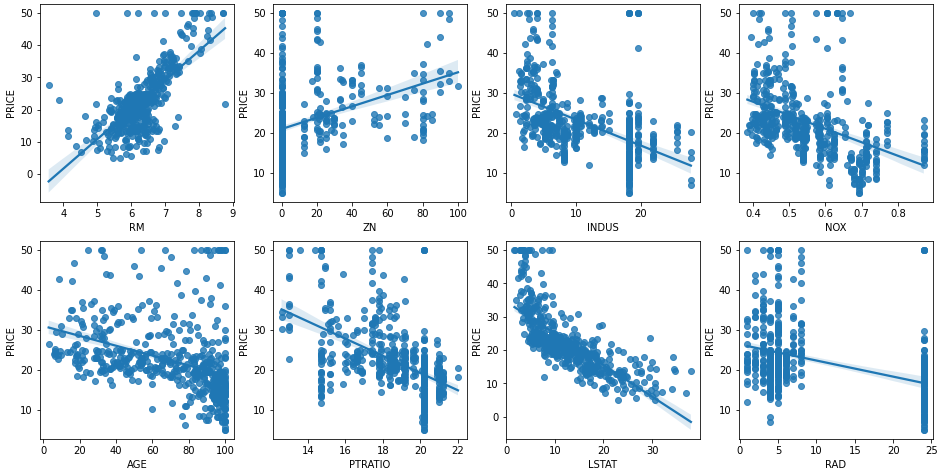

집값 상승과 상관관계 best : RM (방 갯수)
집값 하락과 상관관계 best : LSTAT (하위계층 비율)

사이킷런 train, test 분리하고 학습/예측/평가 수행

506개 데이터 -> 7:3 train/test 데이터 분리
train : 학습 -> linear regression 학습/모델링 수행 -> 모델(W) 생성
test : 평가(validation)-> 평가지표 (MSE, RMSE, ... )

from sklearn.model_selection import train_test_split
from sklearn.linear_model import LinearRegression
from sklearn.metrics import mean_squared_error, r2_score 
        # m_s_e, r2(선형회귀모델 적합도 : 분산값, 1에 가까울수록 적합도 높음)

# feature, target 데이터 분리
y_target = df['PRICE'] # 레이블(종속변수)
X_data = df.drop(['PRICE'], axis=1, inplace=False) # 피처(독립변수)

# train, test 데이터 분리
X_train , X_test , y_train , y_test = train_test_split(X_data , y_target , test_size=0.3, random_state=156)

# Linear Regression 
lr = LinearRegression()

# fit 메소드 학습 : 주어진 데이터로 estimator(사이킷런이 제공) 알고리즘 학습 
lr.fit(X_train, y_train)

LinearRegression()

print(X_train.shape, X_test.shape)

(354, 13) (152, 13)

# predict 메소드 : 학습된 모델로 예측을 수행
y_preds = lr.predict(X_test) 
y_preds[0:5]

array([23.15424087, 19.65590246, 36.42005168, 19.96705124, 32.40150641])

# rmse를 활용한 평가
mse = mean_squared_error(y_test, y_preds)
rmse = np.sqrt(mse)

print(f'MSE : {mse:.3f}, RMSE: {rmse:.3f}')
print(f'Variance score : {r2_score(y_test, y_preds):.3f}')

MSE : 17.297, RMSE: 4.159
Variance score : 0.757

-> Variance score, Rw score는 회귀 모델이 데이타를 얼마나 잘 설명하는지를 의미한다.

print("절편 값:", lr.intercept_) # y축 절편값

# 회귀 계수(coefficient) : 독립변수의 변화에 따라 종속변수에 미치는 영향력이 크기
print("회귀계수:", np.round(lr.coef_,1))  

절편 값: 40.99559517216429
회귀계수: [ -0.1   0.1   0.    3.  -19.8   3.4   0.   -1.7   0.4  -0.   -0.9   0.
  -0.6]

# 회귀계수 정렬 (내림차순, 큰 값부터)
coeff = pd.Series(data=np.round(lr.coef_, 1), index=X_data.columns)
coeff.sort_values(ascending=False)

RM          3.4
CHAS        3.0
RAD         0.4
ZN          0.1
INDUS       0.0
AGE         0.0
TAX        -0.0
B           0.0
CRIM       -0.1
LSTAT      -0.6
PTRATIO    -0.9
DIS        -1.7
NOX       -19.8
dtype: float64

RM의 양의 절대값이 제일 크다.
NOX가 음의 절대값이 너무 크다.

cross_val_score() MSE --> RMSE 구하기

from sklearn.model_selection import cross_val_score

# features, target 데이터 정의 
y_target = df['PRICE']
X_data = df.drop(['PRICE'], axis=1)

# 선형회귀 객체 생성
lr = LinearRegression()
lr

LinearRegression()

# 5 folds 의 개별 Negative MSE scores (음수로 만들어 작은 오류 값이 더 큰 숫자로 인식됨)
neg_mse_scores = cross_val_score(lr, X_data, y_target, scoring="neg_mean_squared_error", cv = 5)
    # cv는 교차검증의 폴드 수
neg_mse_scores

array([-12.46030057, -26.04862111, -33.07413798, -80.76237112,
       -33.31360656])

# RMSE를 구하기 위해선 MSE 값에 -1을 곱한 후 평균을 내면 된다
rmse_scores =  np.sqrt(-1*neg_mse_scores)
rmse_scores
# cross_val_score() # shift + tab, tab 으로 함수 확인

array([3.52991509, 5.10378498, 5.75101191, 8.9867887 , 5.77179405])

# 5 fold 의 평균 RMSE
avg_rmse = np.mean(rmse_scores)
avg_rmse

5.828658946215835

# cross_val_score(scoring="neg_mean_squared_error")로 반환된 값은 모두 음수
print(' 5 folds 의 개별 Negative MSE scores: ', np.round(neg_mse_scores, 2))
print(' 5 folds 의 개별 RMSE scores : ', np.round(rmse_scores, 2))
print(f' 5 folds 의 평균 RMSE : {avg_rmse:.3f}')

 5 folds 의 개별 Negative MSE scores:  [-12.46 -26.05 -33.07 -80.76 -33.31]
 5 folds 의 개별 RMSE scores :  [3.53 5.1  5.75 8.99 5.77]
 5 folds 의 평균 RMSE : 5.829

-> 보스턴 주택가격 예측을 했더니 RMSE가 5.829 나왔다.