[핸즈온 머신러닝] 3. 분류

woneze·2024년 9월 11일

Hands-On Machine Learning

목록 보기

3/18

3.1 MNIST

from sklearn.datasets import fetch_openml

mnist = fetch_openml('mnist_784', as_frame=False)

mnist 로드

X, y = mnist.data, mnist.target

70,000개의 이미지. 784개의 특성.
28 x 28 픽셀의 이미지
각 특성은 0~255까지의 픽셀 강도를 나타냄

import matplotlib.pyplot as plt

def plot_digit(image_data):
  image = image_data.reshape(28, 28)
  plt.imshow(image, cmap="binary")
  plt.axis("off")

some_digit = X[0]
plot_digit(some_digit)
plt.show()

cmap="binary"로 지정하여 0을 흰색, 255를 검은색으로 나타내는 흑백 컬러 맵 사용
숫자 5로 보이는 이 그림의 레이블은 5

X_train, X_test, y_train, y_test = X[:60000], X[60000:], y[:60000], y[60000:]

훈련 세트(앞쪽 60,000개), 테스트 세트(뒤쪽 10,000개)
훈련 세트는 이미 섞여 있음 → 모든 교차 검증 폴드를 비슷하게 만들어 줌

3.2 이진 분류기 훈련

이진 분류기(binary classifier) : target일 경우만 true, 나머지는 모두 false

y_train_5 = (y_train == '5')
y_test_5 = (y_test == '5')

from sklearn.linear_model import SGDClassifier

sgd_clf = SGDClassifier(random_state=42)
sgd_clf.fit(X_train, y_train_5)

sgd_clf.predict([some_digit])

확률적 경사 하강법(Stochastic Gradient Descent, SGD) 분류기로 처리
SGD는 한 번에 하나씩 훈련 샘플을 독립적으로 처리할 수 있어서 온라인 학습에 적합
분류기는 해당 이미지가 5를 나타낸다고 추측(True)

3.3 성능 측정

3.3.1 교차 검증을 사용한 정확도 측정

from sklearn.model_selection import cross_val_score
cross_val_score(sgd_clf, X_train, y_train_5, cv=3, scoring="accuracy")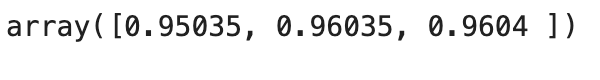

정확도(accuracy)가 모든 교차 검증 폴드에 대해 95% 이상

from sklearn.dummy import DummyClassifier

dummy_clf = DummyClassifier()
dummy_clf.fit(X_train, y_train_5)
print(any(dummy_clf.predict(X_train)))

False가 출력됨. True로 예측된 것이 없음.

cross_val_score(dummy_clf, X_train, y_train_5, cv=3, scoring="accuracy")

정확도가 90% 이상
이미지의 10% 정도가 5이기 때문에 무조건 5가 아니라고 예측해도 정확히 맞출 확률이 90%

3.3.2 오차 행렬

불균형한 테이터셋을 다룰 때, 분류기의 성능을 평가하는 더 좋은 방법은 오차 행렬(confusion matrix)를 조사하는 것

from sklearn.model_selection import cross_val_predict

y_train_pred = cross_val_predict(sgd_clf, X_train, y_train_5, cv=3)

from sklearn.metrics import confusion_matrix
cm = confusion_matrix(y_train_5, y_train_pred)
cm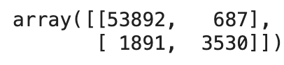

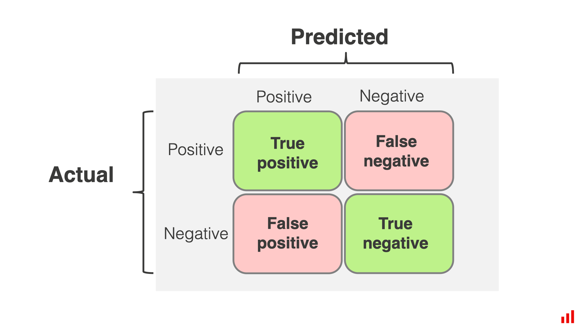
오차 행렬의 행은 실제 클래스, 열은 예측한 클래스
음성 클래스 (negative class) : '아닌 것'을 판별하는 클래스
- 진짜 음성 (true negative) : '아닌 것'을 '아닌 것'으로 잘 판별한 것
- 거짓 양성 (false negative) : '아닌 것'을 '맞는 것'으로 잘못 판별한 것
양성 클래스 (positive class) : '맞는 것'을 판별하는 클래스
- 거짓 음성 (false negative) : '맞는 것'을 '아닌 것'으로 잘못 판별한 것
- 진짜 양성 (true positive) : '맞는 것'을 '맞는 것'으로 잘 판별한 것

3.3.3 정밀도와 재현율

정밀도(precision)

정밀도 = \frac{TP}{TP+FP}

TP : 진짜 양성의 수
FP : 거짓 양성의 수

재현율(recall)

재현율 = \frac{TP}{TP+FN}

FN : 거짓 음성의 수
정밀도와 재현율을 같이 사용하는 것이 일반적임
민감도(sensitivity) 또는 진짜 양성 비율(true positive rate, TPR)이라고도 함

from sklearn.metrics import precision_score, recall_score
precision_score(y_train_5, y_train_pred) # == 3530 / (687 + 3530)
recall_score(y_train_5, y_train_pred) # == 3530 / (1891 + 3530)

F1 score

F_1 = \frac{2}{\frac{1}{정밀도}+\frac{1}{재현율}}=2×\frac{정밀도×재현율}{정밀도+재현율}=\frac{TP}{TP+\frac{FN+FP}{2}}

from sklearn.metrics import f1_score
f1_score(y_train_5, y_train_pred)

F1 score는 정밀도와 재현율의 조화 평균(harmonic mean)
F1 score가 높아지려면 재현율과 정밀도가 모두 높아야 함
상황에 따라 정밀도가 중요할 수도 있고 재현율이 중요할 수도 있음

3.3.4 정밀도/재현율 트레이드오프

정밀도/재현율 트레이드 오프 : 정밀도를 올리면 재현율이 줄고 그 반대도 마찬가지

SGDClassifier

결정 함수(decision function)을 사용하여 각 샘플의 점수를 계산
점수가 결정 임곗값(decision threshold)보다 크면 양성 클래스, 그렇지 않으면 음성 클래스

적절한 임곗값 정하기

from sklearn.metrics import precision_recall_curve

precisions, recalls, thresholds = precision_recall_curve(y_train_5, y_scores)

cross_val_predict() 함수를 이용해 훈련 세트에 있는 모든 샘플의 점수를 구함

from sklearn.metrics import precision_recall_curve

precisions, recalls, thresholds = precision_recall_curve(y_train_5, y_scores)

이전 코드에서 구한 점수를 바탕으로 precision_recall_curve() 함수를 사용하여 가능한 모든 임곗값에 대해 정밀도와 재현율 계산

plt.plot(thresholds, precisions[:-1], "b--", label="Precision", linewidth=2)
plt.plot(thresholds, recalls[:-1], "g--", label="Recall", linewidth=2)
plt.vlines(threshold, 0, 1.0, "k", "dotted", label="Threshold")

idx = (thresholds >= threshold).argmax()
plt.plot(thresholds[idx], precisions[idx], "bo")
plt.plot(thresholds[idx], recalls[idx], "go")
plt.axis([-50000, 50000, 0, 1])
plt.grid()
plt.xlabel("Threshold")
plt.legend(loc="center right")

plt.show()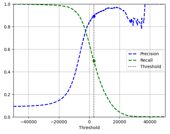

해당하는 임곗값(3,000)에서 정밀도는 약 90%, 재현율은 약 50%

import matplotlib.patches as patches  # 구부러진 화살표를 그리기 위해서

plt.figure(figsize=(6, 5))

plt.plot(recalls, precisions, linewidth=2, label="Precision/Recall curve")

plt.plot([recalls[idx], recalls[idx]], [0., precisions[idx]], "k:")
plt.plot([0.0, recalls[idx]], [precisions[idx], precisions[idx]], "k:")
plt.plot([recalls[idx]], [precisions[idx]], "ko",
         label="Point at threshold 3,000")
plt.gca().add_patch(patches.FancyArrowPatch(
    (0.79, 0.60), (0.61, 0.78),
    connectionstyle="arc3,rad=.2",
    arrowstyle="Simple, tail_width=1.5, head_width=8, head_length=10",
    color="#444444"))
plt.text(0.56, 0.62, "Higher\nthreshold", color="#333333")
plt.xlabel("Recall")
plt.ylabel("Precision")
plt.axis([0, 1, 0, 1])
plt.grid()
plt.legend(loc="lower left")

plt.show()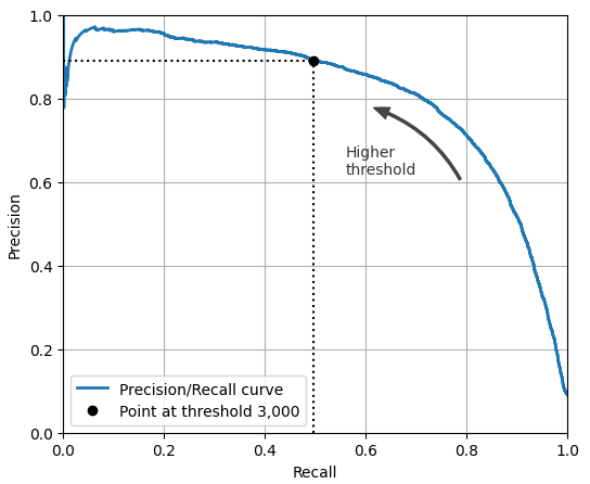

재현율 80% 근처에서 정밀도가 급격하게 줄어드는 양상. 이 하강점 직전을 정밀도/재현율 트레이드오프로 선택하는 것이 좋음.

idx_for_90_precision = (precisions >= 0.90).argmax()
threshold_for_90_precision = thresholds[idx_for_90_precision]
threshold_for_90_precision
# 3370.0194991439557

정밀도가 최소 90%가 되는 가장 낮은 임곗값

y_train_pred_90 = (y_scores >= threshold_for_90_precision)
precision_score(y_train_5, y_train_pred_90)
# 0.9000345901072293

recall_at_90_precision = recall_score(y_train_5, y_train_pred_90)
recall_at_90_precision
# 0.4799852425751706

정밀도 90%를 달성한 분류기를 만들었지만, 재현율 48%는 부족한 값임

3.3.5 ROC 곡선

FPR(false positive rate)에 대한 TPR(true positive rate)의 곡선
FPR은 1에서 TNR(true negative rate)을 뺀 값
TNR을 특이도(specificity)라고도 함
ROC 곡선은 민감도에 대한 1-특이도 그래프

from sklearn.metrics import roc_curve

fpr, tpr, tresholds = roc_curve(y_train_5, y_scores)

idx_for_threshold_at_90 = (thresholds <= threshold_for_90_precision).argmax()
tpr_90, fpr_90 = tpr[idx_for_threshold_at_90], fpr[idx_for_threshold_at_90]

plt.plot(fpr, tpr, linewidth=2, label="ROC curve")
plt.plot([0, 1], [0, 1], 'k:', label="Random classifier's ROC curve")
plt.plot([fpr_90], [tpr_90], "ko", label="Threshold for 90% precision")

plt.gca().add_patch(patches.FancyArrowPatch(
    (0.20, 0.89), (0.07, 0.70),
    connectionstyle="arc3,rad=.4",
    arrowstyle="Simple, tail_width=1.5, head_width=8, head_length=10",
    color="#444444"))
plt.text(0.12, 0.71, "Higher\nthreshold", color="#333333")
plt.xlabel('False Positive Rate (Fall-Out)')
plt.ylabel('True Positive Rate (Recall)')
plt.grid()
plt.axis([0, 1, 0, 1])
plt.legend(loc="lower right", fontsize=13)

plt.show()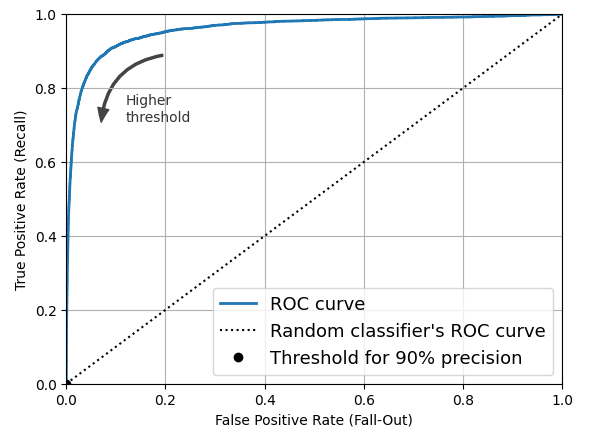

TPR이 높을수록 FPR이 증가
좋은 분류기는 점선에서 멀리 떨어져야 함(왼쪽 위로)
AUC(area under the curve) 측정을 통해 분류기들을 비교할 수 있음

from sklearn.ensemble import RandomForestClassifier

forest_clf = RandomForestClassifier(random_state=42)
y_probas_forest = cross_val_predict(forest_clf, X_train, y_train_5, cv=3,
                                    method="predict_proba")

y_scores_forest = y_probas_forest[:, 1]
precisions_forest, recalls_forest, thresholds_forest = precision_recall_curve(
    y_train_5, y_scores_forest
)

plt.plot(recalls_forest, precisions_forest, "b-", linewidth=2,
         label="Random Forest")
plt.plot(recalls, precisions, "--", linewidth=2, label="SGD")
plt.xlabel("Recall")
plt.ylabel("Precision")
plt.axis([0, 1, 0, 1])
plt.grid()
plt.legend(loc="lower left")

plt.show()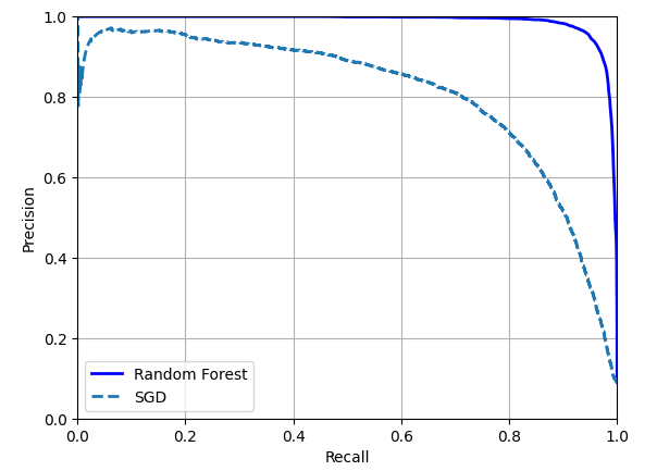

RandomForestClassifier의 PR곡선이 SGDClassifier의 곡선보다 훨씬 더 좋아보임
F1 Score과 ROC AUC 점수도 모두 우수

from sklearn.metrics import roc_auc_score

y_train_pred_forest = y_probas_forest[:, 1] >= 0.5
f1_score(y_train_5, y_train_pred_forest)
# 0.9274509803921569
roc_auc_score(y_train_5, y_scores_forest)
# 0.9983436731328145

3.4 다중 분류

다중 분류기(multiclass classifier)는 둘 이상의 클래스를 구별할 수 있음

이진 분류기를 여러 개 사용해 다중 클래스를 분류하는 기법

OvR(one-versus-the-rest)
- 목표하는 특정 타깃과 나머지를 분류.
- 클래스 N개를 구분하기 위해 분류기 N개를 훈련
- OvA(one-versus-all) 이라고도 함
- ex) 1 ~ 10까지의 숫자 중에서 1만 분류
OvO(one-versus-one)
- 각 조합마다 이진 분류기를 훈련
- 클래스 N개를 구분하기 위해 분류기 N × (N - 1) / 2개를 훈련
- ex) 1 ~ 10까지의 숫자 분류를 위해 0과 1구별, 0과 2 구별, 1과 2 구별 등과 같이 각 숫자의 조합마다 분류기를 훈련

OvO의 장점은 전체 훈련 세트 중 구별할 두 클래스에 해당하는 샘플만 있으면 된다는 점
일부 알고리즘은 OvO를 선호하지만, 대부분의 이진 분류 알고리즘에서는 OvR을 선호함
다중 클래스 분류 작업에 이진 분류 알고리즘을 선택하면 사이킷런이 자동으로 OvR 또는 OvO를 실행함

from sklearn.svm import SVC

svm_clf = SVC(random_state=42)
svm_clf.fit(X_train[:2000], y_train[:2000])

svm_clf.predict([some_digit])
# array(['5'], dtype=object)

some_digit_scores = svm_clf.decision_function([some_digit])
some_digit_scores.round(2)
# array([[ 3.79,  0.73,  6.06,  8.3 , -0.29,  9.3 ,  1.75,  2.77,  7.21, 4.82]])
# 가장 높은 점수는 9.3이고 클래스 5에 해당함

class_id = some_digit_scores.argmax()
class_id
# 5

svm_clf.classes_
# array(['0', '1', '2', '3', '4', '5', '6', '7', '8', '9'], dtype=object)

svm_clf.classes_[class_id]
# '5'

from sklearn.multiclass import OneVsRestClassifier

ovr_clf = OneVsRestClassifier(SVC(random_state=42))
ovr_clf.fit(X_train[:2000], y_train[:2000])

ovr_clf.predict([some_digit])
# array(['5'], dtype='<U1')

len(ovr_clf.estimators_)
# 10
# 10개의 분류기가 훈련되었음

sgd_clf = SGDClassifier(random_state=42)
sgd_clf.fit(X_train, y_train)
sgd_clf.predict([some_digit])
# array(['3'], dtype='<U1')

sgd_clf.decision_function([some_digit]).round()
# array([[-31893., -34420.,  -9531.,   1824., -22320.,  -1386., -26189., -16148.,  -4604., -12051.]])

cross_val_score(sgd_clf, X_train, y_train, cv=3, scoring="accuracy")
# array([0.87365, 0.85835, 0.8689])

from sklearn.preprocessing import StandardScaler
scaler = StandardScaler()
X_trian_scaled = scaler.fit_transform(X_train.astype("float64"))
cross_val_score(sgd_clf, X_train_scaled, y_train, cv=3, scoring="accuracy")
# array([0.8983, 0.891, 0.9018])

SVC 기반으로 OvR 전략을 강제하여 만든 다중 분류기
SGDClassifier를 훈련하고 예측을 만들었음
some_digit에 대해서는 '3'으로 예측을 잘못함 (정답은 '5')
전체 테스트 폴드에 대해서는 85.8% 이상의 성능을 보임
입력의 scale을 조정하여 정확도를 89% 이상으로 높임

3.5 오류 분석

from sklearn.metrics import ConfusionMatrixDisplay

y_train_pred = cross_val_predict(sgd_clf, X_train,scaled, y_train, cv=3)
ConfusionMatrixDisplay.from_predictions(y_train, y_train_pred)
plt.show()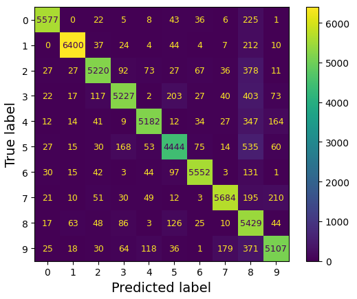

대부분의 이미지가 주대각선에 위치함 = 이미지가 올바르게 분류됨
모델이 5에서 더 많은 오류를 범했거나 데이터 집합에 다른 숫자보다 5가 적기 떄문에 5번 행과 5번 열의 대각선에 있는 셀은 다른 숫자보다 약간 더 어둡게 보임 → 정규화로 해결

ConfusionMatrixDisplay.from_predictions(y_train, y_train_pred,
                                        normalize="true", values_format=".0%")
plt.show()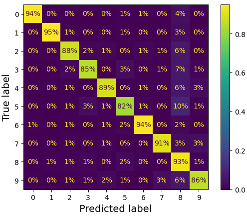

각 값을 해당 클래스의 총 이미지 수로 나누어 오차 행렬을 정규화 (normalize="true")
'5' 중에서 82%가 올바르게 분류됨
가장 많은 오류는 '8'으로 잘못 분류한 것 (10%)

sample_weight = (y_train_pred != y_train)
ConfusionMatrixDisplay.from_predictions(y_train, y_train_pred,
                                        sample_weight=sample_weight,
                                        normalize="true", values_format=".0%")
plt.show()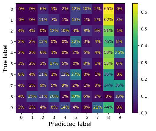

올바른 예측에 대한 가중치를 0으로 하여 오류가 더 눈에 띄도록 함
많은 이미지가 '8'으로 잘못 분류되었음을 알 수 있음
이 그래프에서는 올바른 예측이 제외되어 있음. 1행 9열의 경우 '0'이미지에서 발생한 오류 중 65%가 '8'으로 잘못 분류되었다는 의미임

sample_weight = (y_train_pred != y_train)
ConfusionMatrixDisplay.from_predictions(y_train, y_train_pred,
                                        sample_weight=sample_weight,
                                        normalize="pred", values_format=".0%")
plt.show()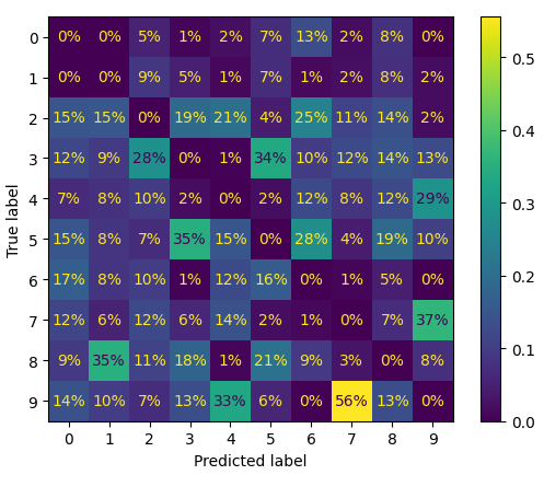

오차 행렬을 열 단위로 정규화

오차 행렬을 분석하면 분류기의 성능 향상 방안에 관한 인사이트를 얻을 수 있음

cl_a, cl_b = '3', '5'
X_aa = X_train[(y_train ==cl_a) & (y_train_pred == cl_a)]
X_ab = X_train[(y_train ==cl_a) & (y_train_pred == cl_b)]
X_ba = X_train[(y_train ==cl_b) & (y_train_pred == cl_a)]
X_bb = X_train[(y_train ==cl_b) & (y_train_pred == cl_b)]

size = 5
pad = 0.2
plt.figure(figsize=(size, size))
for images, (label_col, label_row) in [(X_ba, (0, 0)), (X_bb, (1, 0)),
                                       (X_aa, (0, 1)), (X_ab, (1, 1))]:
    for idx, image_data in enumerate(images[:size*size]):
        x = idx % size + label_col * (size + pad)
        y = idx // size + label_row * (size + pad)
        plt.imshow(image_data.reshape(28, 28), cmap="binary",
                   extent=(x, x + 1, y, y + 1))
plt.xticks([size / 2, size + pad + size / 2], [str(cl_a), str(cl_b)])
plt.yticks([size / 2, size + pad + size / 2], [str(cl_b), str(cl_a)])
plt.plot([size + pad / 2, size + pad / 2], [0, 2 * size + pad], "k:")
plt.plot([0, 2 * size + pad], [size + pad / 2, size + pad / 2], "k:")
plt.axis([0, 2 * size + pad, 0, 2 * size + pad])
plt.xlabel("Predicted label")
plt.ylabel("True label")

plt.show()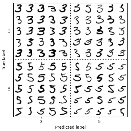

3과 5는 매우 비슷한 모양을 가진 숫자라 오류가 많이 발생함
분류기는 이미지의 위치나 회전 방향에 매우 민감함
이미지를 중앙에 위치시키고 회전되어 있지 않도록 전처리하면 성능 향상을 기대할 수 있음
데이터 증식(data augmentation) : 훈련 이미지를 약간 이동시키거나 회전된 변형 이미지로 훈련 집합을 보강하는 방식

3.6 다중 레이블 분류

다중 레이블 분류 시스템(multilabel classification) : 여러 개의 이진 label을 출력하는 분류 시스템

import numpy as np
from sklearn.neighbors import KNeighborsClassifier

y_train_large = (y_train >= '7')
y_train_odd = (y_train.astype('int8') % 2 == 1)
y_multilabel = np.c_[y_train_large, y_train_odd]
knn_clf = KNeighborsClassifier()
knn_clf.fit(X_train, y_multilabel)

knn_clf.predict([some_digit])
# array([[False, True]])

y_train_knn_pred = cross_val_predict(knn_clf, X_train, y_multilabel, cv=3)
f1_score(y_multilabel, y_train_knn_pred, average="macro")
# 0.976410265560605

이 코드는 모든 레이블의 가중치가 같다고 가정함
multilabel의 첫 번째 값은 7보다 큰 값인지 나타내고 두 번째는 홀수인지 나타냄
숫자 5는 크지 않고(False), 홀수(True)임 → 알맞게 분류

레이블에 클래스의 지지도(타깃 레이블에 속한 샘플 수)를 가중치로 설정하면, 레이블에 속한 데이터의 수가 다른 경우에 생기는 문제를 방지할 수 있음.

from sklearn.multioutput import ClassifierChain

chain_clf = ClassifierChain(SVC(), cv=3, random_state=42)
chain_clf.fit(X_train[:2000], y_multilabel[:2000])

chain_clf.predict([some_digit])
# array([[0., 1.]])

ClassifierChain 클래스를 사용해 예측을 한 코드임
SVC와 같이 기본적으로 다중 레이블 분류를 지원하지 않는 경우 레이블당 하나의 모델을 학습시킬 수 있음. 하지만 레이블 간의 의존성을 포착하기 어려움
큰 수(7, 8, 9)는 짝수일 확률보다 홀수일 확률이 2배 더 높지만 '홀수' 레이블에 대한 분류기는 '큰 값' 레이블 분류기가 무엇을 예측했는지 알 수 없음 → 모델을 체인으로 구성함으로써 해결 가능.

3.7 다중 출력 분류

다중 출력 다중 클래스 분류(multioutput-multiclass classification) : 다중 레이블 분류에서 한 레이블이 다중 클래스가 될 수 있도록 일반화한 것

noise가 많은 숫자 이미지를 입력으로 받아 깨끗한 숫자 이미지를 배열로 출력
분류기의 출력이 다중 레이블(픽셀당 한 레이블)이고 각 레이블은 값을 여러 개 가짐(0~255) → 다중 출력 분류 시스템

np.random.seed(42)
noise = np.random.randint(0, 100, (len(X_train), 784))
X_train_mod = X_train + noise
noise = np.random.randint(0, 100, (len(X_test), 784))
X_test_mod = X_test + noise
y_train_mod = X_train
y_test_mod = X_test

plt.subplot(121); plot_digit(X_test_mod[0])
plt.subplot(122); plot_digit(y_test_mod[0])

plt.show()

randint() 함수를 사용하여 픽셀 강도에 noise 추가
target 이미지는 원본 이미지
좌 : noise 추가한 이미지 / 우 : 원본 이미지

knn_clf = KNeighborsClassifier()
knn_clf.fit(X_train_mod, y_train_mod)
clean_digit = knn_clf.predict([X_test_mod[0]])
plot_digit(clean_digit)
plt.show()