Sobel Edge detection 기초

• Edge Detection은 이미지 픽셀값 사이의 변화량을 이용하여 이미지의 경계선을 계산하는 방법
• 이미지 에서 특정영역을 구분 짓는 방법 중 하나로 활용 됨

Sobel detection

• Sobel dection은 kernel을 활용하여 컨볼루션 연산을 하는 방법이다.
• 중심 픽셀을 기준으로 앞,뒤 픽셀간의 차를 구하여 변화량을 추출
• 이때 중심값에는 가중치로 2를 곱해준다.

Sobel()

dst = cv.Sobel(src, ddepth, dx, dy[, dst[, ksize[, scale[, delta[, borderType]]]]])

dst: 출력 이미지는 입력이미지와 크기 및 채널 수가 동일
The function has 4 required arguments:
1. src: 입력 이미지.
2. ddepth: 출력 되는 이미지의 자료형
3. dx: X방향으로 미분차수
4. dy: Y방향으로 미분차수

OpenCV Documentation

sobel()

소스코드 구현

• 모듈 및 이미지 불러오기

import cv2
from matplotlib import pyplot as plt
import numpy as np

bagpipe = cv2.imread('gene.jpg')

# Convert to grayscale.
bagpipe_gray = cv2.cvtColor(bagpipe, cv2.COLOR_BGR2GRAY)

plt.imshow(bagpipe_gray, cmap = 'gray'); plt.axis('off'); plt.title('original')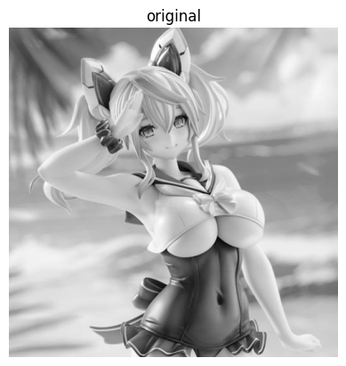

• sobel edge dection 구현

sobelx  = cv2.Sobel(src = bagpipe_gray, ddepth = cv2.CV_64F, dx = 1, dy = 0, ksize = 3) 
sobely  = cv2.Sobel(src = bagpipe_gray, ddepth = cv2.CV_64F, dx = 0, dy = 1, ksize = 3)
sobelxy = sobelx + sobely


plt.figure(figsize= (20,20))
plt.subplot(131);plt.imshow(sobelx, cmap = 'gray'); plt.axis('off'); plt.title('X direction')
plt.subplot(132);plt.imshow(sobely, cmap = 'gray'); plt.axis('off'); plt.title('Y direction')
plt.subplot(133);plt.imshow(sobelxy, cmap = 'gray'); plt.axis('off'); plt.title('X+Y sum')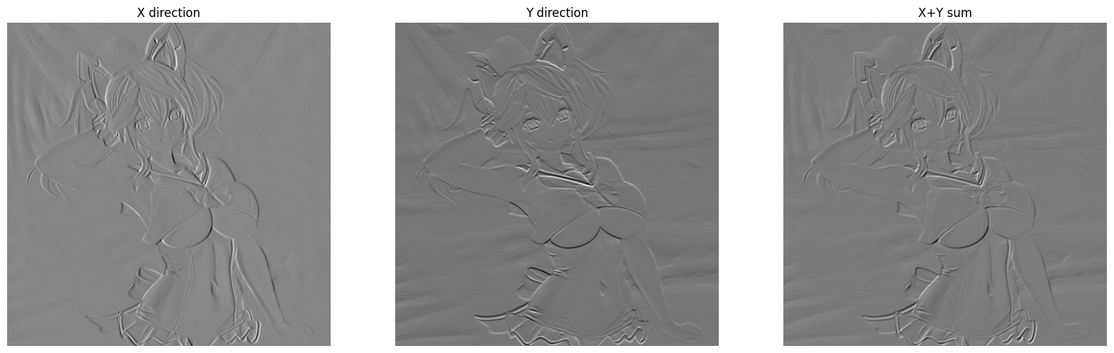

• X방향 연산을 진행하면 Y축에 평행하는 엣지가 검출
• Y방향 연산시 X축에 평행한 엣지가 검출 됨
• 둘을 합하면 원본이미지에서 검출 된 엣지와 유사하게 나타남
• 기울기 값이 양수일 경우에는 흰색으로 표현되고, 음의 값일 경우 검은색으로 표시

Sobel detection with image blur

• 경계선 검출시 이미지의 노이즈가 있는 경우 엣지값이 왜곡이 되는 경우가 있어 노이즈로 발생하는 부분이 있음
• 이를 방지하고 엣지 검출영역의 값을 블러링 하기 위해 가우시안 커널을 사용함

bagpipe_gray_blur = cv2.GaussianBlur(bagpipe_gray,(25,25),1,1)
plt.figure(figsize= (20,20))
plt.subplot(131);plt.imshow(bagpipe_gray, cmap = 'gray'); plt.axis('off'); plt.title('original')
plt.subplot(132);plt.imshow(bagpipe_gray_blur, cmap = 'gray'); plt.axis('off'); plt.title('blur')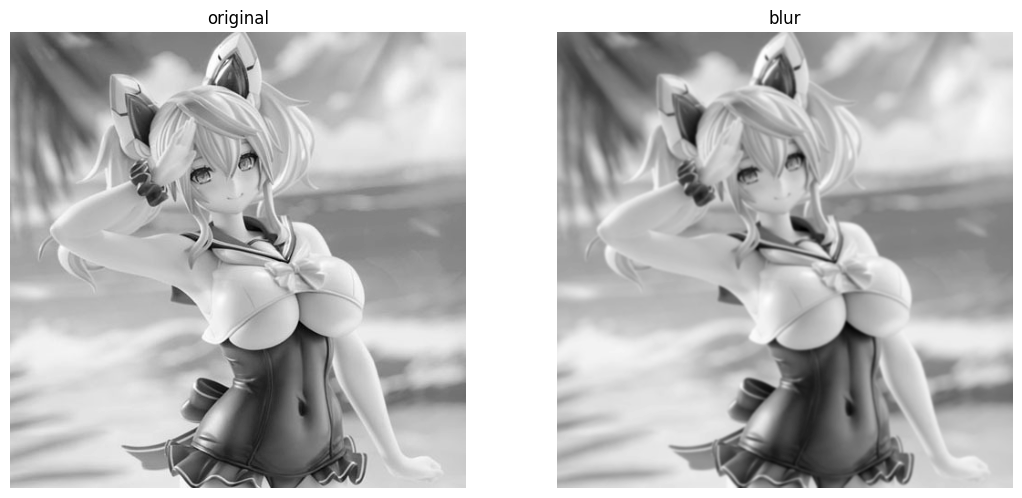

bagpipe_gray_blur = cv2.GaussianBlur(bagpipe_gray,(25,25),1,1)
plt.figure(figsize= (20,20))
plt.subplot(131);plt.imshow(bagpipe_gray, cmap = 'gray'); plt.axis('off'); plt.title('original')
plt.subplot(132);plt.imshow(bagpipe_gray_blur, cmap = 'gray'); plt.axis('off'); plt.title('blur')

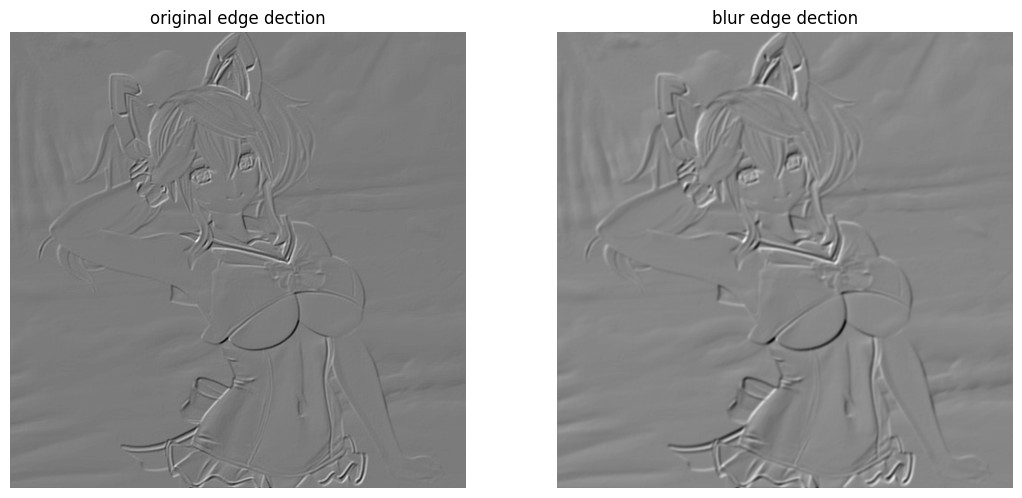
• 이미지 블러 효과를 활용하면 엣지검출시 좀더 선명한 값을 얻을 수 있음