Joint distribution optimal transportation for domain adaptation(NIPS 2017)

Motivation

• 기존의 optimal transport for unsupervised DA 방법론들은 label을 제외한 source sample X만을 transport 시키고 있음
• 이러한 방법론들은 다음의 conditional distribution에 대한 성질이 성립함을 함축적으로 가정함. 즉,$P_s(Y|\mathcal{T}(X)) = P_t(Y|X)$
  - $\mathcal{T}$는 OT mapping of sample
  - $\hat{P_t}(Y|X_t) = Model(Y|\mathcal{T}(X_s)) \sim P_S(Y|T(X_s))$ <- 기존의 OT 방법이 성립하려면 이 가정을 따라야만 합리적임.
• 다만, 기존의 OT mapping 에서는 이 가정이 굳이 성립해야 할 특별한 이유는 없음
• Proposal : Source와 Target의 결합분포를 Transport 시킨다:
  ㄴ 이렇게 하면 위의 문제점이 해결 되는가???
  ㄴ Target의 label 정보를 우리가 모르기 때문에 문제가 되고, 해결방안을 제시하고 있음.
  

JDOT

Kantorovich formulation을 응용하면, 제안하는 방식은 다음과 같은 식으로 나타내어진다.

$\gamma_0 = \arg\min_{\gamma \in \Pi(\mathcal{P}_s, \mathcal{P}_t)} \int_{(\Omega \times \mathcal{C})^2} \mathcal{D}(x_1, y_1; x_2, y_2)d\gamma(x_1, y_1;x_2, y_2)$
where
$\mathcal{D}(x_1, y_1; x_2, y_2) = \alpha d(x_1, x_2) + \mathcal{L}(y_1, y_2)$

위 식의 해(최적의 $\gamma$)는 $\mathcal{D}$가 lower-semi continuous 일 때 존재함이 알려져 있다. (Supp. A 참고) 이 상황은 $d$가 norm이고 $\mathcal{L}$이 일반적 loss일때 만족된다.

문제는, target data의 label은 우리가 알 수 없다는 점인데,
우리의 목적은 target data에 대하여 잘 동작하는 classifier f를 찾는 것이라는 것을 상기하자. 이를 이용하여, target의 label $y_t \sim f(x_t)$로 근사시키자.(아마 f는 sample 분포에서 학습된 classifier일 것이다).
그리고 근사된 joint distribution $\mathcal{P}_t^f = (X_t, f(X_t))$ 로 적도록 하자.

위의 문제를 empirical distribution과 $\mathcal{P}_t^f$에 대하여 다시 쓰면
$\min_{f, \gamma} \sum_{ij} \mathcal{D}(x_i^s, y_i^s; x_t^s, f(x_t))\gamma_{ij} = \min W(\mathcal{P_s}, \mathcal{P_t^f})$.

현실에서는, f의 overfitting 방지를 위해 f에 추가적인 제약조건이 걸리기도 한다.

Comparison with other OT based DA methods

• JDOT에서는 굳이 barycentric mapping을 찾을 필요가 없음
  ㄴ 직접 f를 구하려고 시도하기 때문.
  ㄴ barycentric mapping은 두 분포 사이에 wasserstein distance를 근사적으로 줄일 뿐이므로, 이론적 배경이 JDOT에 비해 부족함

A bound on the target error

JDOT를 통해 구해진 f에 대한 이론적 성질을 보인다.

Notation
$f \in \mathcal{H}$ : hypothesis in hypothesis space
$err_T(f) = E_{(x,y) \sim P_t}(\mathcal{L}(y,f(x)))$

Assumption
$\mathcal{L}$은 Bounded, symmetric, k-lipschitz이며 triagular ineq.을 만족함을 가정

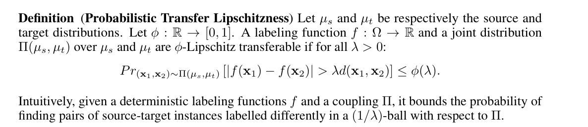
또한, 기존 lipschitz 조건의 확장인 probabilistic lipschitz라는 개념을 도입한다.

f가 prob.libschitzness를 만족한다는 것은, 가까운 두 객체가 비슷한 함수값을 높은 확률로 가진다는 것을 모델링 할 수 있다.

Main theorem

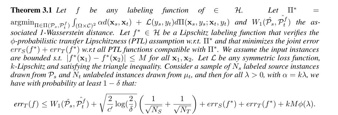
(증명은 supp.B에 적어둔다)
의미를 해석해보자.

• $f \in \mathcal{H}$는 임의의 labeling function.
• $\Pi^*$는 $\mathcal{P}_s, \mathcal{P}_t^f$ 사이의 optimal coupling.
• $f^*$는 다음 조건 만족
  ㄴ Lipschitz labeling function
  ㄴ $\Pi^*$에 대해$\phi$ probabilistic transfer lipschitzness 만족
  ㄴ 위 조건 만족시키는 f 중 $err_s(f^*) + err_T(f^*)$를 최소화시킴
  ㄴ $\forall x_1, x_2, |f(x_1) - f(x_2)| \leq M$ for some $M >0$
• $\mathcal{L}$ : symmetric, k-lipschitz, satifies triangle ineq.

즉, $W_1(\hat\mathcal{P}_s, \hat\mathcal{P}_t^f)$를 최소화함으로서, $err_T(f)$가 작아진다는 의미이다.

Learning with JDOT

다음과 같은 setting을 고려한다

• $f \in \mathcal{H}$는 RKHS or Parameterized 될 수 있는 함수들의 집합이다.
  ㄴ 이러한 함수 클래스는 linear model, NN, kernel methods 등을 포함함.
• regularization term $\Omega(f)$
  ㄴ 주로 squared norm 에 대한 비감소 함수.
• 추가적으로 $\gamma$에 대한 regularization도 생각할 수 있다
  ㄴ entropic / group-lasso...
• $\mathcal{L}$은 continuous / differentiable

풀어야 하는 최적화 문제는 다음과 같다.

$\min_{f \in \mathcal{H}, \gamma \in \Delta}\sum_{i,j}\gamma_{ij}(\alpha d(x_s^i, x_t^j) + \mathcal{L}(y_s^i, f(x_t^j)) + \lambda\Omega(f)$

Optimization procedure

• $\gamma$ 와 $f$에 대해서 따로따로 최소화시키는 것이 가장 일반적인 방법이다
  ㄴ Block Coordinate Descent(BCD) or Gauss-Seidel Method

• $f$ 가 고정되어 있는 경우, 이는 classical OT문제가 되며
  ㄴ network simplex algorithm / regularized OT / stochastic OT.. 등으로 풀 수 있다.

• $\gamma$ 가 고정되어 있는 경우,
  $\min_{f \in \mathcal{H}, \gamma \in \Delta}\sum_{i,j}\gamma_{ij} \mathcal{L}(y_s^i, f(x_t^j)) + \lambda\Omega(f)$ 와 같은 식을 최적화 하는 문제
  ㄴ $N_sN_t$개의 항을 가지므로 computationally expensive
  ㄴ Loss를 잘 고르면 complexity 줄일 수 있다.(추후 설명)
  ㄴ$\mathcal{H}$ 가 RKHS일 때, represeneter theorem에 의하면, 위와 같은 최적화 문제의 해는 $f^* = \sum_i^{N_t}\alpha_i K(x_i, x)$의 형태로 표현되고, 즉 $N_t$개의 parameter을 최적화시키는 문제가 된다.
  ㄴ 2-block Gauss-Seidel method로 최적화 가능하다고 한다.

Supplementary materials

A. optimal $\gamma_0$의 존재성

$\gamma_0 = \arg\min_{\gamma \in \Pi(\mathcal{P}_s, \mathcal{P}_t)} \int_{(\Omega \times \mathcal{C})^2} \mathcal{D}(x_1, y_1; x_2, y_2)d\gamma(x_1, y_1;x_2, y_2)$

B. Proof of the main theorem

(업데이트 예정)