< Prophet >

• 페이스북에서 공개한 시계열 예측 라이브러리

---

• 주요 구성 요소는 총 4가지로

1. Trend 2. Seasonality 3. Holiday 4. 오차

• Trend : 주기적이지 않은 변화 트렌드
• Seasonality : weekly, yearly 등 주기적으로 나타나는 패턴
• Holiday : 불규칙한 이벤트.
  (특정 기간에 값이 비정상적으로 증가 또는 감소하는 경우 holiday로 정의)
• 오차 : 정규분포를 따르는 잔차

---

Example 1

import pandas as pd 
import numpy as np 
import matplotlib.pyplot as plt 
%matplotlib inline 


time = np.linspace(0, 1, 365*2)
result = np.sin(2*np.pi*12*time)
ds = pd.date_range("2023-01-01", periods=365*2, freq="D")
df = pd.DataFrame({"ds": ds, "y": result})
df.head()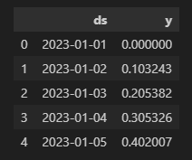

df["y"].plot(figsize=(10, 6));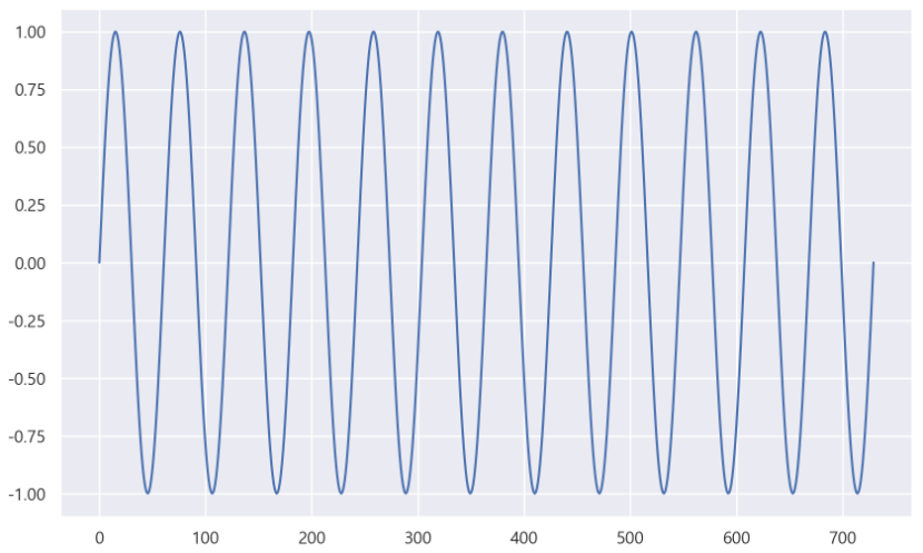

import prophet

m = prophet.Prophet(yearly_seasonality=True, daily_seasonality=True)
m.fit(df);

• 예측값을 넣을 데이터 프레임 생성
  ( periods 값은 향후 몇일을 예측할 것인지 설정 )
  
  
  

future = m.make_future_dataframe(periods=30)
forecast = m.predict(future)
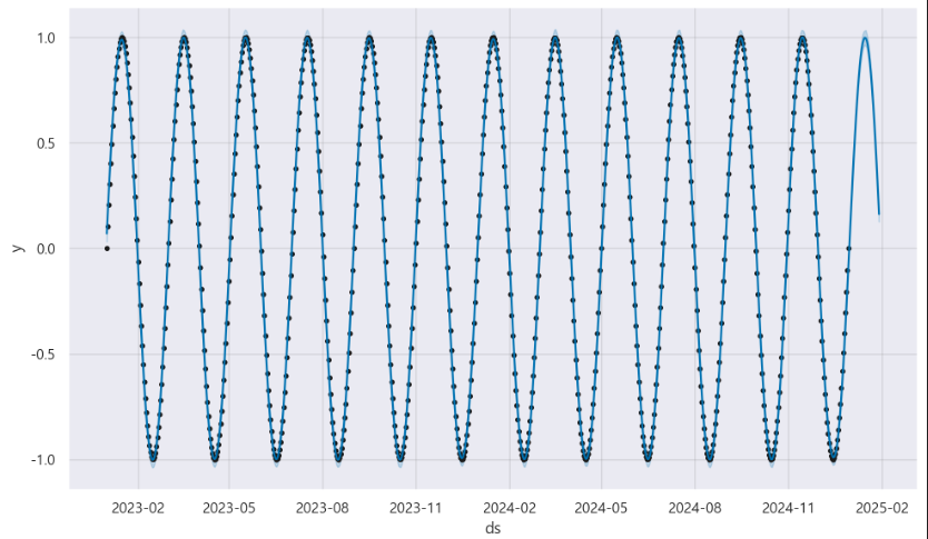
m.plot(forecast);

예측 결과 시각화

• 파란색 선이 모델이 예측한 값
• 검정색 점이 실제 데이터 값

Example 2

ㄴ time 추가

time = np.linspace(0, 1, 365*2)
result = np.sin(2*np.pi*12*time) + time 

ds = pd.date_range("2023-01-01", periods=365*2, freq="D")
df = pd.DataFrame({"ds": ds, "y": result})

df["y"].plot(figsize=(10, 6));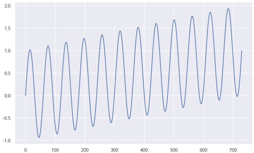

m = prophet.Prophet(yearly_seasonality=True, daily_seasonality=True)
m.fit(df)
future = m.make_future_dataframe(periods=30)
forecast = m.predict(future)
m.plot(forecast);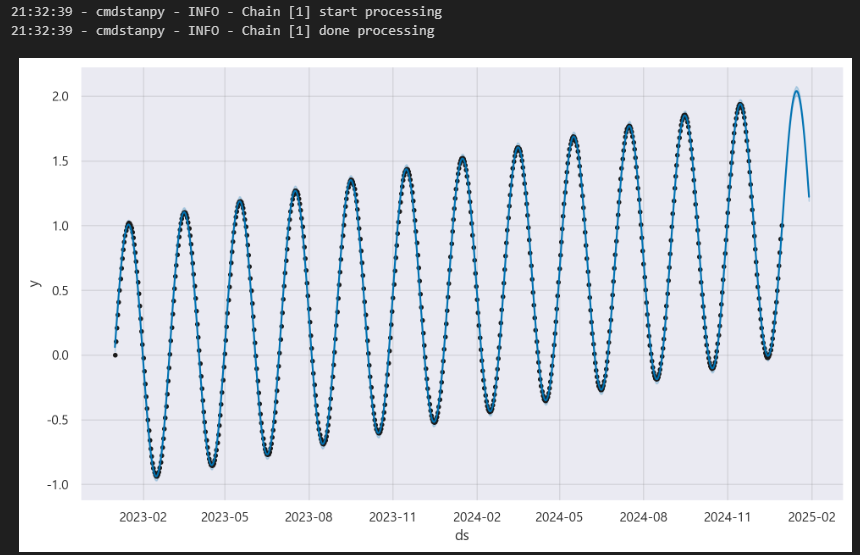

Example 3

ㄴ Holiday 고려

time = np.linspace(0, 1, 365*2)
result = np.sin(2*np.pi*12*time) + time + np.random.randn(365*2)/4

ds = pd.date_range("2023-01-01", periods=365*2, freq="D")
df = pd.DataFrame({"ds": ds, "y": result})

df["y"].plot(figsize=(10, 6));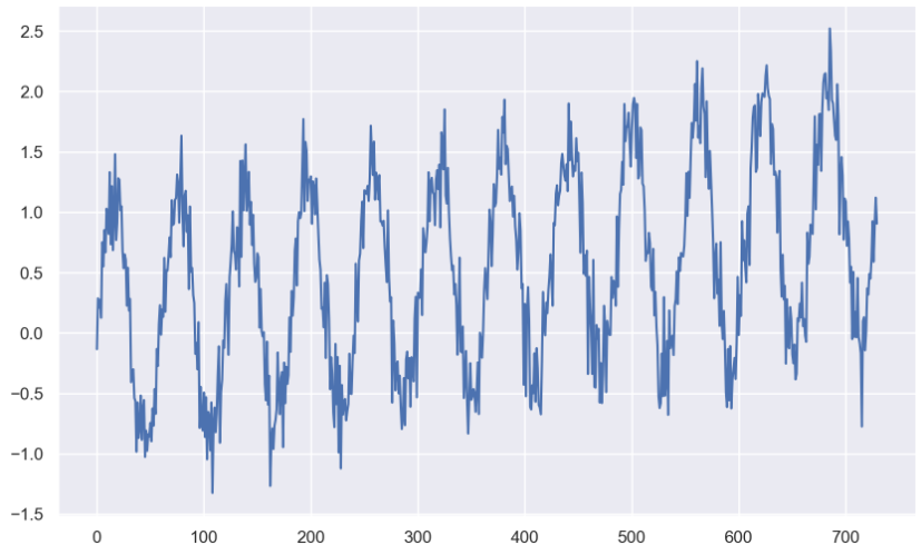

m = prophet.Prophet(yearly_seasonality=True, daily_seasonality=True)
m.fit(df)
future = m.make_future_dataframe(periods=30)
forecast = m.predict(future)
m.plot(forecast);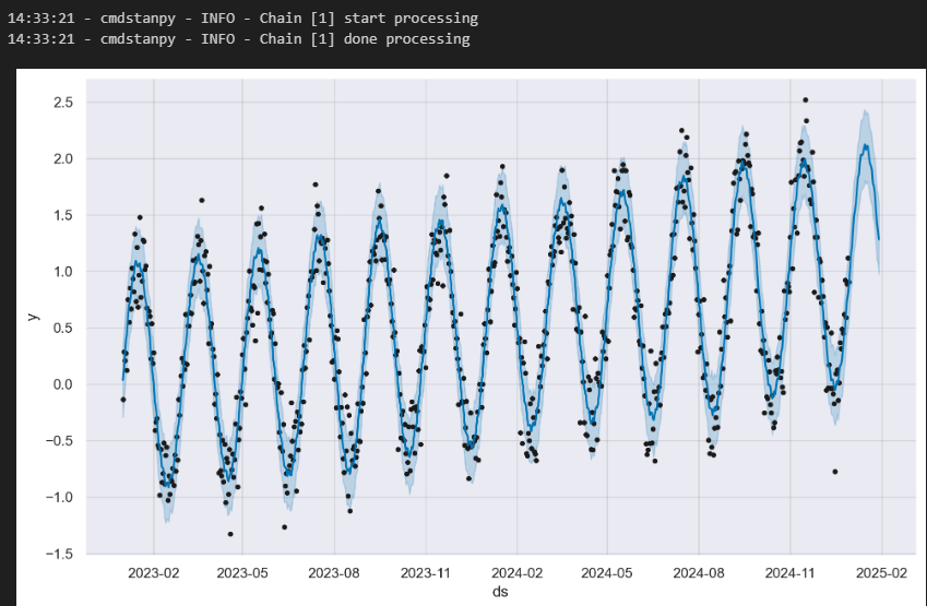

Example 4

ㄴ 잔차 고려

# data name -> pinkwink_web

pinkwink_web["hit"].plot(figsize=(12, 4), grid=True);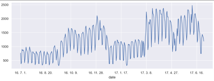

• trend 분석을 시각화하기 위한 x축 값 만들기

time = np.arange(0, len(pinkwink_web))
traffic = pinkwink_web["hit"].values
fx = np.linspace(0, time[-1], 1000)

• 에러를 계산할 함수 작성

def error(f, x, y):
    return np.sqrt(np.mean((f(x) - y) ** 2))
    

fp1 = np.polyfit(time, traffic, 1)
f1 = np.poly1d(fp1)

f2p = np.polyfit(time, traffic, 2)
f2 = np.poly1d(f2p)

f3p = np.polyfit(time, traffic, 3)
f3 = np.poly1d(f3p)

f15p = np.polyfit(time, traffic, 15)
f15 = np.poly1d(f15p)



plt.figure(figsize=(12, 4))
plt.scatter(time, traffic, s=10)
plt.plot(fx, f1(fx), lw=4, label='f1')
plt.plot(fx, f2(fx), lw=4, label='f2')
plt.plot(fx, f3(fx), lw=4, label='f3')
plt.plot(fx, f15(fx), lw=4, label='f15')

plt.grid(True, linestyle="-", color="0.75")
plt.legend(loc=2)
plt.show()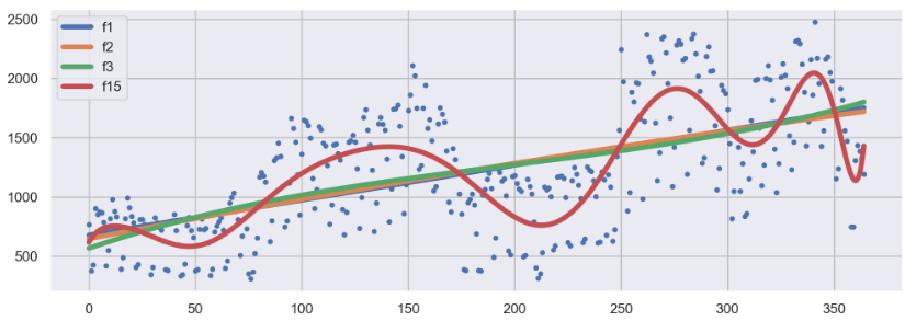

m = prophet.Prophet(yearly_seasonality=True, daily_seasonality=True)
m.fit(df);

# 60일에 해당하는 데이터 예측 
future = m.make_future_dataframe(periods=60)

# 예측 결과는 상한/하한의 범위를 포함해서 얻어진다 
forecast = m.predict(future)
forecast[["ds", "yhat", "yhat_lower", "yhat_upper"]].tail()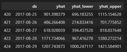

m.plot(forecast);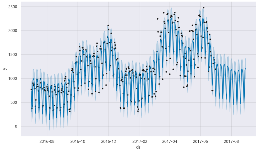

m.plot_components(forecast);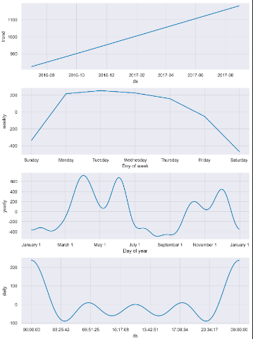

• Trend는 점점 증가하는 추세
• 주 계절성은 월요일부터 크게 증가, 금요일부터는 하락세
• 연 계절성은 4월, 6월에 특히 높은 상승을 보임.