1. 개요

• 주어진 버섯특성 데이터 2개
  • mushroom_train.csv(6500건)
  • mushroom_test.csv(1624건)
• train 데이터를 학습시켜서 test데이터의 독성/식용을 판단하는 프로젝트

2. 프로젝트 진행방향

• 버섯 특성 및 독성판단 여부 파악
• 데이터 전처리 작업
  - 결측치 해결
  • 삭제항목, 결합항목 선별
  • 범주형, 서열형 데이터 파악 및 처리
  • 각종 통계 적용 데이터 분산 및 상관관계 파악

3. 버섯 특성 및 독성관련 파악

-

버섯 데이터 속성 정보(Attribute Information)

(classes: edible=e, poisonous=p)**
. cap-shape: bell=b,conical=c,convex=x,flat=f,knobbed=k,sunken=s
. cap-surface: fibrous=f,grooves=g,scaly=y,smooth=scap-color: . brown=n,buff=b,cinnamon=c,gray=g,green=r,pink=p,purple=u,red=e,white=w,yellow=y
. bruises: bruises=t,no=f
. odor: almond=a,anise=l,creosote=c,fishy=y,foul=f,musty=m,none=n,pungen. t=p,spicy=s
. gill-attachment: attached=a,descending=d,free=f,notched=n
. gill-spacing: close=c,crowded=w,distant=d
. gill-size: broad=b,narrow=n
. gill-color: black=k,brown=n,buff=b,chocolate=h,gray=g,green=r,orange=o,pink=p,purple=u,red=e,white=w,yellow=y
. stalk-shape: enlarging=e,tapering=t
. stalk-root: bulbous=b,club=c,cup=u,equal=e,rhizomorphs=z,rooted=r,missing=?
. stalk-surface-above-ring: fibrous=f,scaly=y,silky=k,smooth=s
. stalk-surface-below-ring: fibrous=f,scaly=y,silky=k,smooth=s
. stalk-color-above-ring: brown=n,buff=b,cinnamon=c,gray=g,orange=o,pink=p,red=e,white=w,yellow=y
. stalk-color-below-ring: brown=n,buff=b,cinnamon=c,gray=g,orange=o,pink=p,red=e,white=w,yellow=y
. veil-type: partial=p,universal=u
. veil-color: brown=n,orange=o,white=w,yellow=y
. ring-number: none=n,one=o,two=t
. ring-type: cobwebby=c,evanescent=e,flaring=f,large=l,none=n,pendant=p,sheathing=s,zone=z
. spore-print-color: black=k,brown=n,buff=b,chocolate=h,green=r,orange=o,purple=u,white=w,yellow=y
. population: abundant=a,clustered=c,numerous=n,scattered=s,several=v,solitary=y
. habitat: grasses=g,leaves=l,meadows=m,paths=p,urban=u,waste=w,woods=d

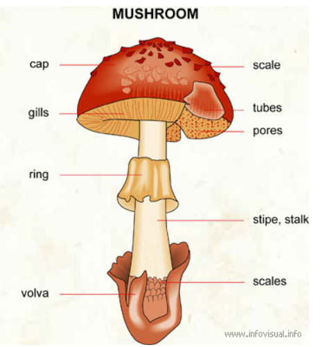
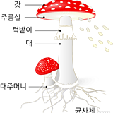
버섯 명칭 이해

cap-shape(Feature / Categorical) = 버섯 갓 모양
cap-surface(Feature / Categorical) = 버섯 갓 표면
cap-color(Feature / Binary)= 버섯 갓 색깔
bruises(Feature / Categorical) = 버섯의 멍?
odor(Feature / Categorical) = 냄새
gill-attachment (Feature / Categorical) = 주름살 부착
gill-spacing(Feature / Categorical) = 주름살 간격
gill-size(Feature / Categorical) = 주름살 사이즈
gill-color(Feature / Categorical) = 주름살 색
stalk-shape(Feature / Categorical) = 대 모양
stalk-root(Feature / Categorical) = 대 뿌리
stalk-surface-above-ring(Feature / Categorical) = 턱받이 위의 대 표면
stalk-surface-below-ring(Feature / Categorical) = 턱받이 아래의 대 표면
stalk-color-above-ring(Feature / Categorical) = 턱받이 위 대 색깔
stalk-color-below-ring(Feature / Categorical) = 턱받이 아래 대 색깔
veil-type(Feature / Binary) = 베일(: 신부 면사포 같이 생긴것) 타입
veil-color(Feature / Categorical) = 베일 색깔
ring-number(Feature / Categorical) = 턱받이 수
ring-type(Feature / Categorical) = 턱받이 타입
spore-print-color(Feature / Categorical) = 버섯 기공(피부의 구멍과 같은) 색깔
population(Feature / Categorical) = 버섯이 얼마나 흔한지(개체수)
habitat(Feature / Categorical) = 서식지-

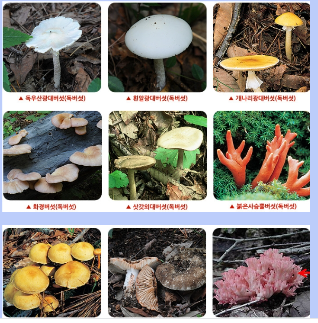
독버섯 상식

독버섯에 대한 이것 저것
색갈이 화사한 노란, 붉은, 자주, 황금싸리버섯 등은 독성이 있다.
아마톡신을 가진 독우산광대버섯, 흰알광대버섯, 개나리광대버섯이
가장 잘알려져 있고, 유럽지역에서는 알광대버섯이 치명적인
독버섯 중독사고를 일으키고 있어요.
일본에서는 화경버섯과 삿갓외대버섯이 독버섯 중독사고를 가장
많이 일으키고, 사망사고를 일으키는 독버섯은 독우산광대버섯,
흰알광대버섯, 붉은사슴뿔버섯, 노란다발, 절구버섯아재비 등.
이들 버섯류는 우리나라에서도 자주 발견되는 버섯들입니다
특히 모양이 아름답고 화려한 색상의 버섯은 독 버섯이 많습니다.
<일반적인 독버섯의 감별법>
1. 악취가 나는 것은 유독하다
2. 빛깔이 진하고 아름다운 것은 유독하다
3. 줄기에 턱이 있는 것은 유독하다
4. 유즙을 분비하는 것은 유독하다
5. 버섯을 물에 넣고 끓일 때 은수저를 검게 변화시키는 것은 유독하다.
그러나 예외도 많아 특별한 주의가 요구된다.

4. 데이터 전처리 작업

1) 열 삭제 및 병합대상 항목파악

• gill-attachment: 대다수가 'f' 동일값
• stalk-root: mushroom_train에 "?" 포함 946건, 비포함 5554건 mushroom_test에 "?" 포함 1534건, 미포함 90건
  5.87%만 테스트케이스에 존재함
• stalk-surface-above-ring & stalk-surface-below-ring
• stalk-color-above-ring & stalk-color-below-ring
  각각 성격이 같기에 합쳐서 처리, df["AB"] = df["A"] + df["B"]
• veil-은 제거 .... 다른 사례들 게시글 참조
• 버섯독성 관련 3개를 선정 dummy화: cap-shape, odor, cap-color 항목. 그런데 너무 항목이 늘어나기에 칼러같은 경우 y,r,u 가타 하면 좋은듯. 독버섯 색상이 노란, 붉은, 자주색 -- test중에 영향요소가 큰 3개로 변경
• 3개 통계상 영향이 큰 3개로 변경 'spore-print-color': 피부 구멍같이 버섯 기공의 색깔, 'gill-size': 주름의 크기, odor: 냄새

spore-print-color
w 2388
n 1968
k 1872
h 1632
r 72
u 48
o 48
y 48
b 48

gill-size
b 5612
n 2512

odor
n 3528
f 2160
y 576
s 576
a 400
l 400
p 256
c 192
m 36

gill-attachment
f 7914
a 210

stalk-root # 테스트케이스에는 90건만 데이터 존재, 1534건은 "?" 값
b 3776
? 2480
e 1120
c 556
r 192

• train.csv logical file name "df"
  df.columns
  Index(['mushroom_id', 'class', 'cap-shape', 'cap-surface', 'cap-color',
  'bruises', 'odor', 'gill-attachment', 'gill-spacing', 'gill-size',
  'gill-color', 'stalk-shape', 'stalk-root', 'stalk-surface-above-ring',
  'stalk-surface-below-ring', 'stalk-color-above-ring',
  'stalk-color-below-ring', 'veil-type', 'veil-color', 'ring-number',
  'ring-type', 'spore-print-color', 'population', 'habitat'],
  dtype='object')
  
• test.csv logical file name "df1"
  df1.columns

Index(['mushroom_id', 'cap-shape', 'cap-surface', 'cap-color', 'bruises',
'odor', 'gill-attachment', 'gill-spacing', 'gill-size', 'gill-color',
'stalk-shape', 'stalk-root', 'stalk-surface-above-ring',
'stalk-surface-below-ring', 'stalk-color-above-ring',
'stalk-color-below-ring', 'veil-type', 'veil-color', 'ring-number',
'ring-type', 'spore-print-color', 'population', 'habitat'],
dtype='object')

• 2개의 파일을 하나로 합침
  . df1없는 class항목 'NaN'값 넣어서 생성
  . df1.insert(1,"class","NaN") #항목 순서에 동일 위치에 추가
  . all_df = pd.concat([df, df1]) #df, df1을 all_df하나의 파일로
• all_df['XXX'].value_counts() 각열에 항목값 파악

![](https://velog.velcdn.com/images/wsk527kr/post/b1bd0279-e245-45d0-b0fd-e488005d321f/image.png

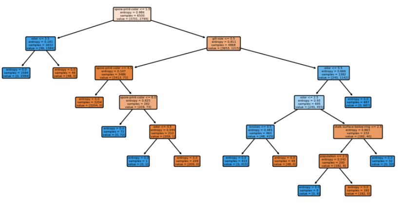
• 생성된 탐색트리 모양
  

• train 데이터 케이스에 독성 버섯과의 관계

버섯냄새
sns.boxplot(
x="class",
y="odor",
data=df_train,
).set(
title="test boxplot"
)

버섯모자 형태
sns.boxplot(
x="class",
y="cap-shape",
data=df_train,
).set(
title="test boxplot"
)

버섯모자 색깔

_ 삭제한 열
veil-color

• stalk-root : 식용에만 관련이 있어 보임
  

Decision Tree
학습 데이터 셋을 종속 변수와 독립 변수로 분리
dftrain = all_df[:6500]
df_test = all_df[6500:]
y_train = df_train["class"]
x_train = df_train.drop(["mushroom_id", "class"], axis=1)
x_test = df_test.drop(["mushroom_id", "class"], axis=1)
DecisionTree 기반 분류 모델 생성 및 학습
from sklearn.tree import DecisionTreeClassifier
decision_tree_clf = DecisionTreeClassifier(criterion='entropy', random_state=42)
decision_tree_clf.fit(x_train, y_train)
Decision Tree 시각화하기
from sklearn.tree import plot_tree
from matplotlib import pyplot as plt
feature_names= x_train.columns.to_list()
plt.figure(figsize=(30,10))
= plot_tree(
decision_tree_clf,
feature_names = feature_names,
filled=True,
rounded=True
)

Feature Importance
importances = decisiontree_clf.feature_importances
importances
import numpy as np
indices = np.argsort(importances)
sorted_feature_names = [feature_names[i] for i in indices]

Create plot

plt.figure()
plt.title("Feature Importance")
ticks = range(len(feature_names))
plt.barh(ticks, importances[indices], align="center")
plt.yticks(ticks, sorted_feature_names)
plt.ylabel("Features")
plt.xlabel("Importance Score")
plt.tight_layout()
plt.show()

5. 학습된 모델 추출

y_test = decision_tree_clf.predict(x_test)
y_test
df_test["class"] = y_test
df_test[["mushroom_id", "class"]].to_csv("./data/very_first_test_Y&O.csv", index=False)
🌴Random Forest
Random Forst 모델 학습시키기
import pandas as pd
df = pd.read_csv('./data/second_all_df.csv')
df_train = df[:6500]
df_test = df[6500:]
y_train = df_train["class"]
x_train = df_train.drop(["mushroom_id", "class"], axis=1)
x_test = df_test.drop(["mushroom_id", "class" ], axis=1)
from sklearn.model_selection import cross_val_score, KFold
kf = KFold(n_splits=5, shuffle=True, random_state=1234)
from sklearn.ensemble import RandomForestClassifier
model = RandomForestClassifier(
n_estimators=10,
criterion="entropy",
max_depth=5,
random_state=1234
)
scores = cross_val_score(model, x_train, y_train, cv=kf)
scores, scores.mean()

Random Forest의 각 Decision Tree가 어떻게 학습되었는지 확인
from matplotlib import pyplot as plt
from sklearn.tree import plottree
plt.figure(figsize=(15,5))
= plottree(
model.estimators[3],
feature_names=x_train.columns,
filled=True,
rounded=True,
fontsize=5
)
Hyper Paramter Optimization 기법 사용
from sklearn.model_selection import GridSearchCV
param_grid = {
"n_estimators": [10, 30, 50],
"max_depth": [3, 5, 10],
"max_features": [3, 5, 9]
}
grid_search = GridSearchCV(
estimator=model,
param_grid=param_grid,
cv=stratified_kf
)
grid_search.fit(x_train, y_train)

학습된 모델 추출
y_test = model.predict(x_test)
df_test["class"] = y_test
df_test[["mushroom_id", "class"]].to_csv("./data/Randomprocess_Y&O.csv", index=False)
👻인사이트
1) Lable Encoding과 Random Forest를 사용했을 때 예측 결과가 1이 되었다.
2) 독버섯을 구분할 때, 버섯의 색과 향이 큰 영향을 미칠 줄 알았지만 bruises, gill-size 등 다양한 변수에 의해 결정된다는 것을 배웠다.
3) 마트에서 파는 새송이버섯과 표고버섯이 짱이다.

🫠한계점

히트맵으로 버섯의 식용 여부와 상관성을 확인해 보니, feature importance와 사뭇 다른 양상을 보여 한편으론 신기했지만 다른 한편으론 식용여부에 더 많은 영향을 미치는 판단 도구로서 무엇을 사용해야 하는지 더 공부해 봐야 할 것 같다