1. 이미지 인식하는 원리
1-1. 데이터 확인하기
from tensorflow.keras.datasets import mnist # MNIST 데이터 불러오기

# 이미지 데이터 : X , 0~9 사이의 이름표 : y
(X_train, y_train), (X_test, y_test) = mnist.load_data()
print('학습셋 이미지수: %d개' %(X_train.shape[0]))
print('테스트셋 이미지수: %d개' %(X_test.shape[0]))

print('X_train의 shape : ', X_train.shape)
print('y_train의 shape : ', y_train.shape)
print('X_test의 shape : ', X_test.shape)
print('y_test의 shape : ', y_test.shape)

# 학습셋 이미지수: 60000개
# 테스트셋 이미지수: 10000개
# X_train의 shape :  (60000, 28, 28)
# y_train의 shape :  (60000,)
# X_test의 shape :  (10000, 28, 28)
# y_test의 shape :  (10000,)
1-2. 첫 번째 이미지 확인하기
# 불러온 이미지중 한 개만 불러오기

import matplotlib.pyplot as plt
plt.imshow(X_train[0], cmap='Greys')
plt.show()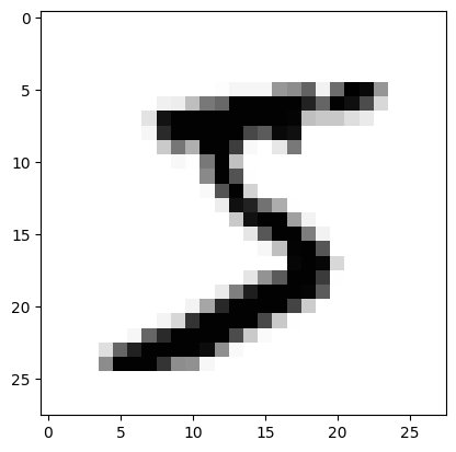
1-3. 이미지가 인식되는 원리
- 숫자 이미지 데이터는 28x28 = 784 픽셀로 이루어져 있다
- 픽셀은 밝기에 따라 0~255 까지 등급을 매긴다
- 흰색 배경 : 0 | 글씨가 들어간 곳 : 1~255
import sys

for x in X_train[0]:
    for y in x:
        sys.stdout.write('%-3s ' %y)
    sys.stdout.write('\n')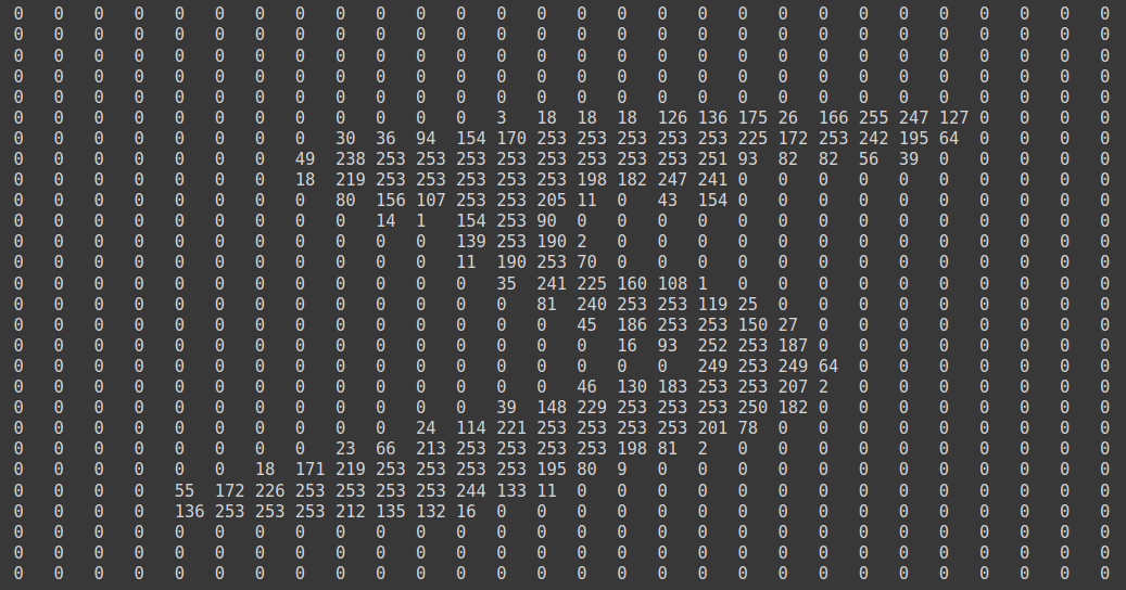
1-4. 데이터 정규화 (차원 변환 과정)
- 이미지가 숫자의 집합으로 바뀌어 학습셋으로 사용된다
- 속성을 담은 데이터를 딥러닝에 집어넣고 클래시를 예측하는 문제로 전환하기
- 28x28=784개의 속성을 이용해 0~9 클래스 열 개 중 하나를 맞히는 문제
- 주어진 가로28, 세로28의 2차원 배열을 784개의 1차원 배열로 바꾸어야 함
- reshape()함수 사용하기 : reshape(총 샘플 수, 1차원 속성의 개수)
- 총 샘플수 : X_train.shape[0] , 1차원 속성의 개수 : 784개
- 케라스는 데이터를 0에서 1사이의 값으로 변환한 후 구동할 때 최적의 성능을 보임
- 현재 0~255 사이의 값으로 이루어진 값을 0~1 사이의 값으로 바꾸어야 함
- 현재 데이터는 0~255사이의 정수로, 정규화를 위해 255로 나누어주려면 먼저 실수형으로 바꾸어야함
# 데이터 차원 바꾸기
X_train = X_train.reshape(X_train.shape[0], 784)
print('차원 바꾼 후 X_train shape :', X_train.shape) # 차원 바꾼 후 X_train shape : (60000, 784)

#데이터 정규화하기
X_train = X_train.astype('float64')
X_train = X_train / 255

# 테스트 데이터도 정규화해주기
X_test = X_test.reshape(X_test.shape[0], 784).astype('float64') / 255

# 숫자 이미지에 새겨진 이름 확인해보기 ( 이전에 불러왔던 이미지 데이터는 5였음, 이 라벨 값은 무엇인지 확인하기)
print("class : %d " % y_train[0]) # class : 5
불러온 X_train[0]의 이미지 데이터 : 5
실제 라벨 값 y_train[0] : 5
1-5. 원핫인코딩
- 0~9의 정수형 값을 갖는 현재 형태에서 0 or 1로만 이루어진 벡터로 수정해야함
- 예시) 이미지 클래스 [5] => [0,0,0,0,0,1,0,0,0,0]
- np.utils.to_categorical() 사용 : np.untils.to_categorical(클래스, 클래스의 개수)
# 클래스 데이터를 원핫 인코딩 적용시키기
from keras.utils import to_categorical

y_train = to_categorical(y_train, 10)
y_test = to_categorical(y_test, 10)

print(y_train[0]) # [0. 0. 0. 0. 0. 1. 0. 0. 0. 0.]
2. 딥러닝 기본 프레임 만들기
# 실습 : MNIST 손글씨 인식하기
from tensorflow.keras.models import Sequential
from tensorflow.keras.layers import Dense
from tensorflow.keras.callbacks import EarlyStopping, ModelCheckpoint
from tensorflow.keras.datasets import mnist
from tensorflow.keras.utils import to_categorical
import matplotlib.pyplot as plt
import numpy as np
import os
# MNIST 데이터 불러오기
(X_train, y_train), (X_test, y_test) = mnist.load_data()
# 차원 변환 후, 테스트 셋과 학습셋으로 나누기
X_train = X_train.reshape(X_train.shape[0], 784).astype('float32') / 255
X_test = X_test.reshape(X_test.shape[0], 784).astype('float32') / 255
# 클래스 0~9 사이를 0 or 1로 바꾸기 (원핫인코딩)
y_train = to_categorical(y_train, 10)
y_test = to_categorical(y_test, 10)
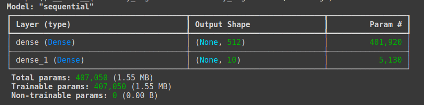
# 모델 구조 설정하기
model = Sequential()
model.add(Dense(512, input_dim=784, activation='relu')) # 이미지 차원이 784로 바뀌어 인풋이 된다
model.add(Dense(10, activation='softmax')) # 출력 값은 0~9사이 값이므로 10개 | 활성화함수는 다중 분류이므로 softmax
model.summary()
# 모델 실행 환경 설정
model.compile(loss='categorical_crossentropy', optimizer='adam', metrics=['accuracy'])
# 모델 최적화를 위한 설정 구간
modelpath = './MNIST_MLP.keras'
checkpointer = ModelCheckpoint(filepath=modelpath, monitor='val_loss', verbose=1, save_best_only=True)
early_stopping_callback = EarlyStopping(monitor='val_loss', patience=10)
#모델 실행
history = model.fit(X_train, y_train, validation_split = 0.25, epochs = 30, batch_size = 200, verbose = 0, callbacks = [early_stopping_callback, checkpointer])
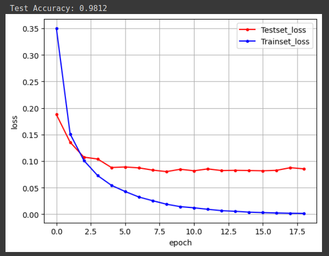
# 테스트 정확도 출력
print('\n Test Accuracy: %.4f' %(model.evaluate(X_test, y_test)[1]))
# 위에서 [1] 을 출력하는 이유 (테스트 데이터의 정확도를 출력하기 위해)
# model.evaluate(X_test, y_test)가 반환하는 리스트에서:
# model.evaluate(X_test, y_test)[0]: 손실 값(loss).
# model.evaluate(X_test, y_test)[1]: 정확도(accuracy)
# 검증셋과 학습셋의 오차 저장
y_vloss = history.history['val_loss']
y_loss = history.history['loss']
# 그래프로 표현
x_len = np.arange(len(y_loss))
plt.plot(x_len, y_vloss, marker='.', c='red', label='Testset_loss')
plt.plot(x_len, y_loss, marker='.', c='blue', label='Trainset_loss')
# 그래프에 그리드를 주고 레이블 표시
plt.legend(loc='upper right')
plt.grid()
plt.xlabel('epoch')
plt.ylabel('loss')
plt.show()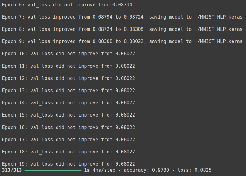
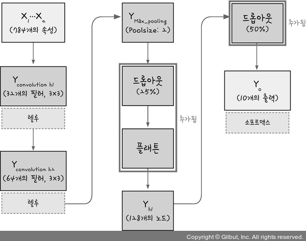
3. 컨볼루션 신경망(CNN)
- 위에서는 은닉층이 하나인 딥러닝 모델로 학습을 시키고 예측 값을 출력하였다
- 이번에는 컨볼루션 신경망을 사용해보기
-
이전 딥러닝에서 했던것 처럼 데이터 정규화 하기
-
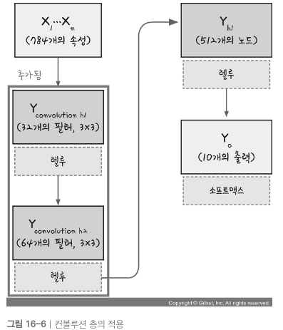
컨볼루션 층을 추가하기 -> 커널(필터)개수, 커널(필터) 크기, 활성화 함수
-
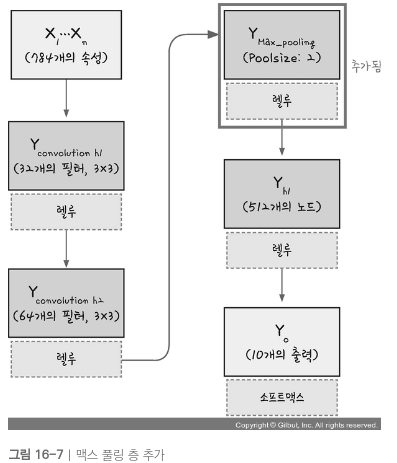
풀링층 추가하기 -> 맥스풀링 or 평균 풀링
-
드롭아웃, 플래튼
- 노드가 많아지거나 층이 많다고해서 학습이 무조건 좋아지지는 않는다
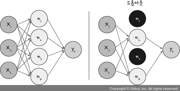
- 과적합을 효과적으로 피해야함
드롭아웃(Drop out): 은닉층에 배치된 노드 중 일부를 임의로 꺼준다- 랜덤하게 노드를 꺼주면 학습 데이터에 지나치게 쳐우혀서 학습되는 과적합을 방지할 수 있음
플래튼(Flatten): 컨볼루션 층과 풀링 층에서는 이미지를 2차원 배열로 다룬다.
이를 1차원 배열로 바꿔야 활성화 함수가 있는 완전 연결층에서 사용할 수 있음
코드 실습
from tensorflow.keras.models import Sequential
from tensorflow.keras.layers import Dense, Dropout, Flatten, Conv2D, MaxPooling2D
from tensorflow.keras.callbacks import ModelCheckpoint, EarlyStopping
from tensorflow.keras.datasets import mnist
from tensorflow.keras.utils import to_categorical

import matplotlib.pyplot as plt
import numpy as np


# 데이터 불러오기

(X_train, y_train), (X_test, y_test) = mnist.load_data()
print('X_train shape:', X_train.shape)
print('X_test shape:', X_test.shape)
print('y_train shape:', y_train.shape)
print('y_test shape:', y_test.shape)

X_train = X_train.reshape(X_train.shape[0], 28, 28, 1).astype('float32') / 255
# (60000,28,28,1) => 60000개의 이미지, 28x28 크기의 픽셀, 채널 = 1 (흑백 : 1, 컬러 : 3)
X_test = X_test.reshape(X_test.shape[0], 28, 28, 1).astype('float32') / 25
y_train = to_categorical(y_train)
y_test = to_categorical(y_test)
print('변경 후 X_train shape:', X_train.shape)
print('변경 후 X_test shape:', X_test.shape)
print('변경 후 y_train shape:', y_train.shape)
print('변경 후 y_test shape:', y_test.shape)


# X_train shape: (60000, 28, 28)
# X_test shape: (10000, 28, 28)
# y_train shape: (60000,)
# y_test shape: (10000,)
# 변경 후 X_train shape: (60000, 28, 28, 1)
# 변경 후 X_test shape: (10000, 28, 28, 1)
# 변경 후 y_train shape: (60000, 10)
# 변경 후 y_test shape: (10000, 10)
데이터 처리 후 X_train 의 데이터는 4차원 배열이 된다.
추가된 마지막 차원 1은채널을 의미하며 흑백 : 1, 컬러 : 3 이다.
CNN 모델에서는 입력 데이터를채널과 함께 처리하므로 4차원으로 바꿔야함
주의할 점
- CNN에서의 4차원 배열과 인풋 형태
- CNN(Convolutional Neural Networks) 모델에서는 입력 데이터가 일반적으로 4차원 배열로 사용됩니다. 그 이유는 모델이 한 번에 여러 샘플(이미지)을 처리하기 때문입니다.
- 첫 번째 차원: 배치 크기(batch size) – 한 번에 처리할 샘플의 수.
- 두 번째 차원: 높이(height) – 이미지의 세로 길이.
- 세 번째 차원: 너비(width) – 이미지의 가로 길이.
- 네 번째 차원: 채널(channels) – 이미지가 흑백인지, RGB(컬러)인지에 따른 채널 수.
하지만, input_shape은 왜 3차원인가?
- input_shape=(28, 28, 1)로 지정된 이유는 개별 이미지의 모양을 지정하는 것이기 때문입니다.
즉, 이 부분에서 배치 크기는 포함하지 않으며, 모델이 각 이미지에 대해 처리할 높이, 너비, 채널을 정의합니다.- 이 input_shape는 배치 크기를 제외한 개별 이미지의 크기를 정의하는 것이므로 3차원으로 설정합니다.
즉, Keras는 배치 크기를자동으로 관리하고, 개별 이미지의 형상만 지정하면 됩니다.
# 컨볼루션 신경망의 설정
model = Sequential()

# 컨볼루션 층 : 32개의 커널(필터), 필터사이즈 : 3x3 , 인풋 shape : 28x28x1, 활성화 함수 : relu
model.add(Conv2D(32, kernel_size=(3, 3), input_shape=(28, 28, 1), activation='relu'))
model.add(Conv2D(64, (3, 3), activation='relu'))

# 맥스풀링 층 : 풀링 사이즈 : 2x2
model.add(MaxPooling2D(pool_size=(2, 2)))
model.add(Dropout(0.25))
model.add(Flatten())
# Flatten 이후에 은닉층인 Dense layer가 추가되는데, 과적합을 방지하기 위해 Dropout을 한 번 더 해준다
model.add(Dense(128, activation='relu'))
model.add(Dropout(0.5))
model.add(Dense(10, activation='softmax'))

model.summary()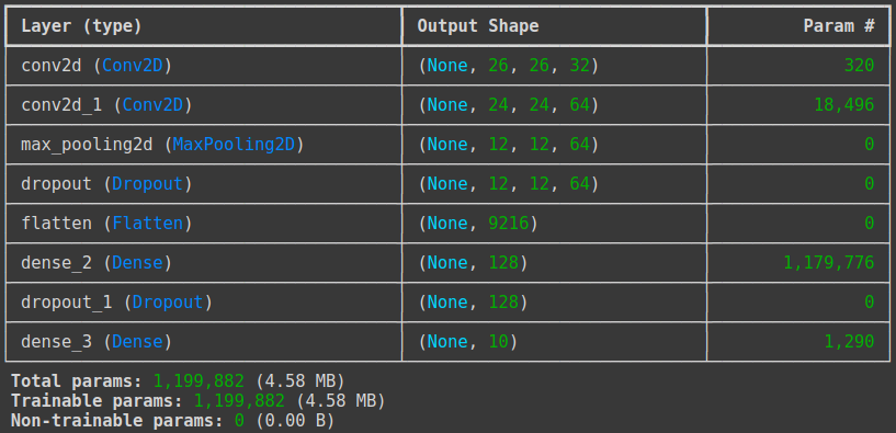
# 모델 실행 옵션 설정
model.compile(loss='categorical_crossentropy', optimizer='adam', metrics=['accuracy'])

# 모델 최적화 설정
modelpath = './MNIST_CNN.keras'
checkpointer = ModelCheckpoint(filepath=modelpath, monitor='val_loss', verbose=1, save_best_only=True)
early_stopping_callback = EarlyStopping(monitor='val_loss', patience=10)

# 모델실행
history = model.fit(X_train, y_train, validation_split=0.25, epochs=30, batch_size=200, verbose=0, callbacks=[early_stopping_callback, checkpointer])

# 테스트 정확도 출력
print('\n Test Accuracy: %.4f' % (model.evaluate(X_test, y_test)[1]))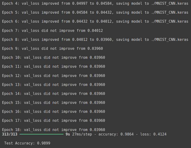
# 검증셋과 학습셋의 오차 저장
y_vloss = history.history['val_loss']
y_loss = history.history['loss']
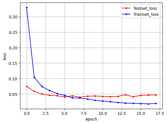
# 그래프로 표현하기
x_len = np.arange(len(y_loss))
plt.plot(x_len, y_vloss, marker='.', c='red', label='Testset_loss')
plt.plot(x_len, y_loss, marker='.', c='blue', label='Trainset_loss')
# 그래프에 그리드를 주고 레이블 표시
plt.legend(loc='upper right')
plt.grid()
plt.xlabel('epoch')
plt.ylabel('loss')
plt.show()
- 기존 딥러닝 학습 결과인 테스트 셋의 정확도 97.8% 보다 CNN 을 사용한 테스트 셋의 정확도 98.99%가 더 높다.
