DL) Cats & Dogs - CNN / ImageDataGenerator / VGG
CNN
1. 데이터 불러오기
import kagglehub
# Download latest version
path = kagglehub.dataset_download("biaiscience/dogs-vs-cats")
print("Path to dataset files:", path)
# r :
Path to dataset files: ...\dogs-vs-cats\versions\1
## 이미지 데이터 경로 설정
import os
path = '.../dogs-vs-cats/versions/1/train/train/'
os.listdir(path)
# r :
['cat.0.jpg',
'cat.1.jpg',
'cat.10.jpg', ... ]
# 인풋 데이터 & 레이블 나누기
full_names = os.listdir(path)
labels = [each.split('.')[0] for each in full_names]
file_id = [each.split('.')[1] for each in full_names]
## 랜덤 이미지 불러오기
import random
import matplotlib.pyplot as plt
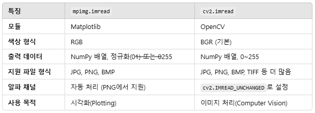
# 이미지를 파일로부터 읽거나 표시하는 데 사용
import matplotlib.image as mpimg
# 이미지 랜덤 선택
sample = random.choice(full_names)
image = mpimg.imread(path+sample)
plt.imshow(image)
plt.show()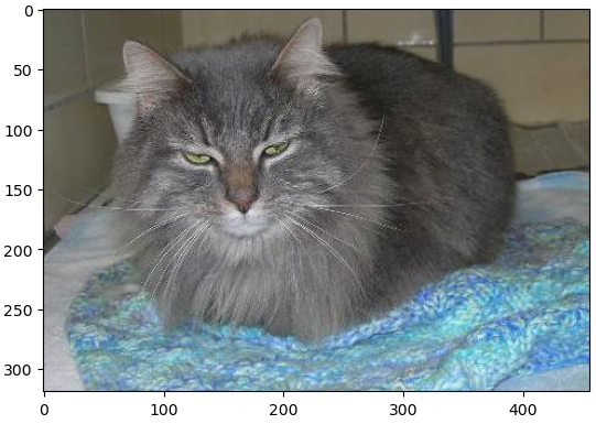
2. 이미지 사이즈 확인
# 다른 이미지 사이즈 확인
sample = random.choice(full_names)
image = mpimg.imread(path+sample)
image.shape

# r :
(305, 398, 3)


## 이미지 리사이즈
from skimage.transform import resize

resized = resize(image, (32,32,3))

fig, axes = plt.subplots(1,2)
axes[0].imshow(image)
axes[1].imshow(resized)
plt.show()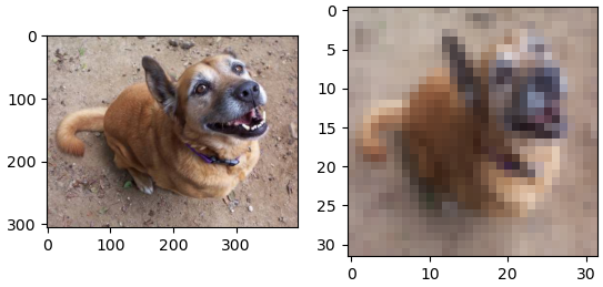
3. 이미지 사이즈 변환 / 인코딩
from tqdm.notebook import tqdm # 진행 상태를 시각적으로 보여주는 모듈
from skimage.color import rgb2gray
import numpy as np

images = []
bar_total = tqdm(full_names)
bar_total = tqdm(full_names, desc="Processing Images")

for each in bar_total:
    image = mpimg.imread(path+each)
    images.append(resize(image, (32,32,3)))

images = np.array(images)
images.shape, labels[:3]

# r
((25000, 32, 32, 3), ['cat', 'cat', 'cat'])

from sklearn.preprocessing import LabelEncoder

# 레이블 인코딩
le = LabelEncoder()
labels_encoded = le.fit_transform(labels)
labels_encoded[:3]

# r :
array([0, 0, 0], dtype=int64)

# 고유 클래스 이름을 오름차순으로 정렬하여 반환
le.classes_

# r :
array(['cat', 'dog'], dtype='<U3')
4. Train 데이터 시각화
from sklearn.model_selection import train_test_split

X_train, X_test, y_train, y_test = train_test_split(images, labels_encoded, test_size=0.2,
                                                   random_state=4, stratify=labels_encoded)

samples = random.choices(population=range(0,20000), k=8)

samples
# r : [17052, 2071, 16385, 643, 893, 9553, 12370, 19462]

plt.figure(figsize=(8,4))

for idx, n in enumerate(samples):
    plt.subplot(2,4,idx+1)
    plt.imshow(X_train[n])
    plt.title(le.classes_[y_train[n]])
    plt.axis('off')
5. 모델 형성 / Compile - CNN 모델
from tensorflow.keras import layers, models

model = models.Sequential([
    layers.Conv2D(32, (3,3), activation='relu', input_shape=(32,32,3)),
    layers.MaxPooling2D((2,2), strides=(2,2)),
    layers.Dropout(0.25),

    layers.Conv2D(64, (3,3), activation='relu', padding='same'),
    layers.MaxPooling2D((2,2), strides=(2,2)),
    layers.Dropout(0.25),

    layers.Conv2D(64, (3,3), activation='relu', padding='same'),
    layers.MaxPooling2D((2,2), strides=(2,2)),
    layers.Dropout(0.25),

    layers.Flatten(),
    layers.Dense(512, activation='relu'),
    layers.Dropout(0.25),
    layers.Dense(2, activation='softmax')
])

model.compile(optimizer='adam', loss='sparse_categorical_crossentropy', metrics=['accuracy'])
6. Train & Evaluate
hist = model.fit(X_train, y_train, epochs=10, verbose=1, validation_data=(X_test, y_test))

# r :
Epoch 10/10
625/625 ━━━━━━━━━━━━━━━━━━━━ 15s 24ms/step - accuracy: 0.7978 - loss: 0.4318 - val_accuracy: 0.8030 - val_loss: 0.4275


plot_target = ['loss', 'val_loss', 'accuracy', 'val_accuracy']

plt.figure()

for each in plot_target:
    plt.plot(hist.history[each], label=each)

plt.legend()
plt.grid()
plt.show()
TensorFlow - ImageDataGenerator
- 메모리 효율적인 데이터 처리
- 데이터셋이 메모리에 한꺼번에 로드하기 어려울 정도로 클 경우, ImageDataGenerator는 배치 단위로 데이터를 실시간으로 생성(on-the-fly)
- 데이터 증강
- 데이터셋이 충분하지 않을 때, 데이터 증강(Augmentation)을 통해 다양한 이미지를 생성
- ex) 이미지 회전, 이동, 확대/축소, 좌우 반전 등을 통해 모델이 더 다양한 상황을 학습
- 증강된 이미지는 원본 데이터의 다양성을 증가시켜 모델의 과적합(Overfitting)을 방지하고 일반화 성능을 높이는 데 도움
- 훈련/검증 데이터 분리
- validation_split 옵션 사용시, 별도의 데이터 분리 작업 없이 subset='training'과 subset='validation'만 설정하면 편리하게 훈련과 검증 데이터를 사용
- 데이터 전처리 자동화
- 이미지 크기 변경(target_size)과 픽셀 값 정규화(rescale=1./255.) 같은 작업을 자동으로 수행
- 대규모 데이터 학습
- 데이터가 많아도, 배치 단위로 처리하면서 실시간으로 데이터를 모델에 공급하기 때문에, 대규모 데이터셋 학습에 적합
1. 클래스 별 폴더 생성
import os
# shutil : 고수준 파일 작업(복사, 이동, 삭제 등)을 제공
import shutil

path = path = '.../train/train/'
classes = ['cat', 'dog']

for class_name in classes:
    class_path = os.path.join(path, class_name)
    # 각 클래스 폴더를 생성
    # exist_ok=True: 폴더가 이미 존재하면 에러를 발생시키지 않고 계속 진행
    os.makedirs(class_path, exist_ok=True)

    for file in full_names:
        if class_name in file:
        	# 조건을 만족하는 파일을 해당 클래스 폴더로 이동
            # os.path.join(path, file): 원본 파일의 전체 경로.
			# os.path.join(class_path, file): 파일이 이동될 대상 클래스 폴더의 전체 경로
            shutil.move(os.path.join(path, file), os.path.join(class_path, file))
2. ImageDataGenerator 생성
# ImageDataGenerator : 이미지 데이터를 실시간으로 변환(augmentation)하거나 전처리(rescaling)하여 학습에 사용할 수 있도록 제너레이터를 생성
from tensorflow.keras.preprocessing.image import ImageDataGenerator

# 이미지 데이터를 0~1 범위로 정규화
# 전체 데이터의 20%를 검증 데이터로 사용
datagen = ImageDataGenerator(
    rescale=1./255. , validation_split=0.2)

# 한 번에 처리할 이미지 배치 크기 (32개의 이미지를 한 번에 처리)
batch_size = 32


# 지정된 디렉터리에서 훈련 데이터를 로드
train_generator = datagen.flow_from_directory(
    path,
    target_size=(128,128),
    batch_size=batch_size,
    class_mode='binary', # 이진 분류를 위해 레이블을 0 또는 1로 변환
    subset='training'
)

# r :
Found 20000 images belonging to 2 classes.

# 검증 데이터를 로드하기 위해 새로운 제너레이터를 생성
validation_generator = datagen.flow_from_directory(
    path,
    target_size=(128,128),
    batch_size=batch_size,
    class_mode='binary',
    subset='validation'
)

# r :
Found 20000 images belonging to 2 classes.
3. Model 형성 / Compile - CNN 모델
from tensorflow.keras import layers, models

model = models.Sequential([
    layers.Conv2D(32, (3,3), activation='relu', input_shape=(128,128,3)),
    layers.MaxPooling2D((2,2), strides=(2,2)),
    layers.Dropout(0.25),

    layers.Conv2D(64, (3,3), activation='relu', padding='same'),
    layers.MaxPooling2D((2,2), strides=(2,2)),
    layers.Dropout(0.25),

    layers.Conv2D(64, (3,3), activation='relu', padding='same'),
    layers.MaxPooling2D((2,2), strides=(2,2)),
    layers.Dropout(0.25),

    layers.Flatten(),
    layers.Dense(512, activation='relu'),
    layers.Dropout(0.25),
    layers.Dense(2, activation='softmax')
])

model.compile(optimizer='adam', loss='sparse_categorical_crossentropy', metrics=['accuracy'])
4. Model Train
model.fit(
    train_generator,
    epochs=5,
    validation_data = validation_generator
)

# r :
Epoch 5/5
625/625 ━━━━━━━━━━━━━━━━━━━━ 339s 542ms/step - accuracy: 0.8173 - loss: 0.3975 - val_accuracy: 0.8663 - val_loss: 0.3210
VGG - 샘플
- 이미지를 OpenCV로 로드하고 RGB 형식으로 변환하여 시각화.
- 이미지를 (224, 224, 3) 크기로 리사이즈하고, 전처리를 통해 모델 입력에 맞게 변환.
- 사전 훈련된 VGG16 모델로 예측 수행.
- decode_predictions로 예측 결과를 해석 가능한 텍스트 형식으로 변환.
- 가장 높은 확률의 클래스 이름과 확률 출력.
1. 모듈 임포트
!pip install opencv-python
!pip install tensorflow

import cv2
from tensorflow.keras.applications.vgg16 import VGG16
from tensorflow.keras.preprocessing.image import img_to_array
from tensorflow.keras.applications.vgg16 import preprocess_input

# TensorFlow Keras에서 제공하는 사전 훈련된 VGG16 모델을 로드하는 명령
model = VGG16(weights='imagenet')
2. VGG16 실행
import matplotlib.pyplot as plt

################################## 이미지 로드

path = ".../Downloads/dog.jpg"

# cv2.imread : 이미지를 BGR 형식으로 읽음
image = cv2.imread(path)


################################## 이미지 시각화

# OpenCV의 BGR 이미지를 RGB 형식으로 변환
# Matplotlib은 이미지를 RGB 형식으로 표시
plt.imshow(cv2.cvtColor(image, cv2.COLOR_BGR2RGB))


################################## 이미지 전처리

# VGG16 모델은 고정된 입력 크기 (224, 224, 3)를 요구
image = cv2.resize(image, (224,224))

# 이미지를 NumPy 배열로 변환
image = img_to_array(image)

# 모델은 4차원 입력 (batch_size, height, width, channels)를 요구
# 이미지 한 장 = 1
image = image.reshape((1, image.shape[0], image.shape[1], image.shape[2]))

# 참고)
image.shape
# r :
(224, 224, 3)

# VGG16 모델의 사전 훈련된 데이터와 일치하도록 이미지를 정규화
image = preprocess_input(image)


################################## 모델 예측

# VGG16 모델을 사용하여 입력 이미지의 클래스 확률을 예측
# 크기 (1, 1000)의 배열이며, 1,000개의 클래스에 대한 확률을 포함
yhat = model.predict(image)
yhat

# r :
array([[8.21378990e-07, 4.65977479e-08, 1.24004655e-08, 1.23889068e-08,
        4.85644698e-08, 2.10464108e-07, 2.84767534e-08, 4.35830657e-07,
        2.40653117e-06, 6.63893829e-08, 2.56418218e-07, 2.69114821e-07,
        2.02008241e-08, 3.51870966e-07, 3.91891462e-07, 1.07186979e-08, ... ]], dtype=float32)

yhat.shape

# r :
(1, 1000)


################################## 결과 디코딩

# 숫자로 된 클래스 인덱스를 사람이 이해할 수 있는 클래스 이름과 확률로 변환
from tensorflow.keras.applications.vgg16 import decode_predictions

label = decode_predictions(yhat)
label

# r :
[[('n02110958', 'pug', 0.82058764),
  ('n03803284', 'muzzle', 0.10120924),
  ('n02099712', 'Labrador_retriever', 0.019212635),
  ('n02104029', 'kuvasz', 0.016876172),
  ('n02112706', 'Brabancon_griffon', 0.004944236)]]

################################## 최상위 클래스 추출

label = label[0][0]
print(label[1], label[2])

# r :
pug 0.82058764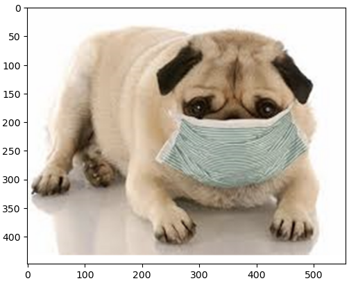
VGG - 함수 적용
1. 데이터 불러오기
import kagglehub

# Download latest version
path = kagglehub.dataset_download("biaiscience/dogs-vs-cats")

print("Path to dataset files:", path)

import os

path = '.../dogs-vs-cats/versions/1/train/train/'

os.listdir(path)

# r :
['cat.0.jpg',
 'cat.1.jpg',
 'cat.10.jpg', ...]

full_names = os.listdir(path)
labels = [each.split('.')[0] for each in full_names]
file_id = [each.split('.')[1] for each in full_names]
2. 모듈 임포트
import random
import matplotlib.image as mpimg
import matplotlib.pyplot as plt
from tensorflow.keras.applications.vgg16 import decode_predictions
import cv2
from tensorflow.keras.utils import img_to_array
from tensorflow.keras.applications.vgg16 import preprocess_input
3. 모델 함수 적용
################################## 함수 정의

def resize_and_preprocess_vgg(image):
    image = cv2.resize(image, dsize=(224,224))
    image = img_to_array(image)
    image = image.reshape((1, image.shape[0], image.shape[1], image.shape[2]))
    image = preprocess_input(image)
    return image

def predict_vgg(image):
    yhat = model.predict(image)
    label = decode_predictions(yhat)
    return label[0][0][1]


################################## 메인 루프

plt.figure(figsize=(8,4))

idx = 1

for each in random.choices(full_names, k=6):
    image = mpimg.imread(path+each)
    plt.subplot(3,2,idx)

    plt.imshow(image)
    idx+=1

    image = resize_and_preprocess_vgg(image)
    result = predict_vgg(image)
    plt.title(result)
    plt.axis('off')

plt.show()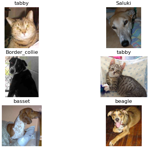
Transfer Learning
1. 모듈 임포트
import tensorflow as tf
import numpy as np
import pandas as pd
import os

from tensorflow.keras.layers import GlobalAveragePooling2D, Dense, Dropout
from tensorflow.keras.models import Sequential
from tensorflow.keras.applications.vgg16 import VGG16, preprocess_input
from tensorflow.keras.preprocessing.image import ImageDataGenerator
2. 데이터 불러오기
path = '.../dogs-vs-cats/versions/1/train/train/'

train_df = pd.DataFrame({'file': os.listdir(path)})

train_df['label'] = train_df['file'].apply(lambda x : x.split('.')[0])
train_df.head()

from sklearn.model_selection import train_test_split

train_data, val_data = train_test_split(train_df, test_size=0.2, stratify=train_df['label'], random_state=4)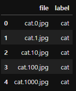
3. ImageDataGenerator
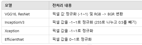
1) preprocessing_function=preprocess_input
- TensorFlow Keras의 사전 학습된 모델에서 제공하는 전처리 함수로, 입력 데이터를 해당 모델이 학습한 데이터와 동일한 방식으로 정규화
- preprocess_input 함수는 모델에 따라 다르게 동작
2) train_datagen.flow_from_dataframe
- flow_from_dataframe은 Keras의 ImageDataGenerator와 함께 사용되며, Pandas 데이터프레임에서 이미지 경로와 레이블 정보를 기반으로 배치 단위로 데이터를 생성하는 함수
- 이미지 경로 (x_col) / 레이블 정보 (y_col).
- 매개변수 class_mode: 레이블 형식 지정
- 'categorical': 원-핫 인코딩된 레이블.
- 'binary': 이진 레이블(0 또는 1).
- 'sparse': 정수 인코딩된 레이블.
- None: 레이블이 없는 경우(예: 예측).
## ImageDataGenerator 설정

# Training Data 설정
train_datagen = ImageDataGenerator(
    rotation_range = 15,
    horizontal_flip = True,
    #  사전 학습된 모델에 적합한 입력으로 데이터를 정규화
    preprocessing_function=preprocess_input)

# Validation Data 설정
# 검증 데이터는 증강하지 않고, 단순히 전처리만 수행
val_datagen = ImageDataGenerator(
    preprocessing_function=preprocess_input)


batch_size=16

# Train Data 생성
train_generator = train_datagen.flow_from_dataframe(
    dataframe=train_data,
    directory=path,
    x_col='file',
    y_col='label',
    # 레이블을 원-핫 인코딩으로 변환. 다중 클래스 분류에 사용
    class_mode='categorical',
    target_size=(224,224),
    batch_size=batch_size,
    seed=13)

# r :
# 총 20,000개의 이미지가 유효하며, 2개의 클래스에 속함
Found 20000 validated image filenames belonging to 2 classes.


# Validation Data 생성
val_generator = val_datagen.flow_from_dataframe(
    dataframe=val_data,
    directory=path,
    x_col='file',
    y_col='label',
    class_mode='categorical',
    target_size=(224,224),
    batch_size=batch_size,
    seed=13,
    # 검증 데이터는 순서가 고정되어 있어야 하므로 데이터를 섞지 않음
	# 이를 통해 예측 결과와 데이터가 올바르게 매칭
    shuffle=False)

# r :
# 총 5,000개의 검증 이미지가 유효하며, 2개의 클래스에 속함
Found 5000 validated image filenames belonging to 2 classes.
4. VGG16 불러오기
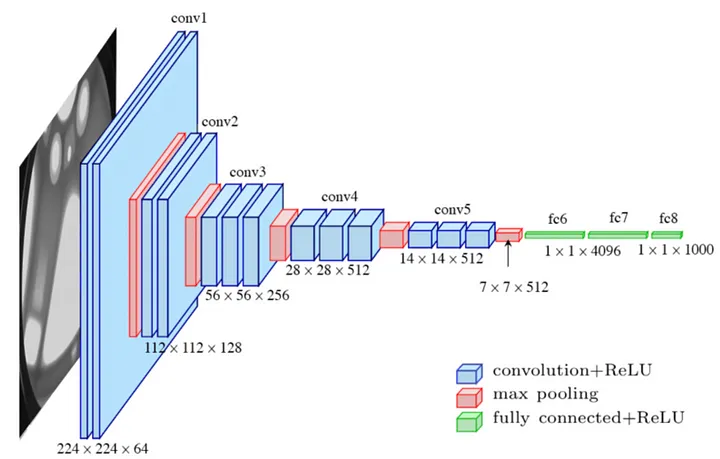
- TensorFlow Keras에서 제공하는 VGG16 모델
- 이 모델은 2014년 ImageNet 챌린지에서 사용된 구조로, 이미지 분류와 같은 작업에 적합
- VGG16 모델의 기본 구조:
- 합성곱 레이어 (Convolutional Layers): 이미지에서 특성을 추출.
- 풀링 레이어 (Pooling Layers): 특성을 압축.
- Fully Connected 레이어 (FC 레이어): 1,000개 클래스에 대한 분류를 수행. - VGG16 참고 설명
VGG16 is composed of 13 convolutional layers, 5 max-pooling layers, and 3 fully connected layers. Therefore, the number of layers having tunable parameters is 16 (13 convolutional layers and 3 fully connected layers). That is the reason why the model name is VGG16. The number of filters in the first block is 64, then this number is doubled in the later blocks until it reaches 512. This model is finished by two fully connected hidden layers and one output layer. The two fully connected layers have the same neuron numbers which are 4096. The output layer consists of 1000 neurons corresponding to the number of categories of the Imagenet dataset.
(출처 : https://lekhuyen.medium.com/an-overview-of-vgg16-and-nin-models-96e4bf398484)
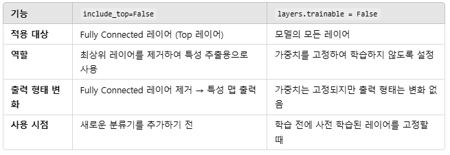
1) include_top = False 의 역할
- VGG16 모델의 Fully Connected(FC) 레이어, 즉 분류를 담당하는 최상위(Top) 레이어를 제거하고, 출력이 마지막 합성곱 레이어의 특성 맵이 되도록 설정
- 제거 전 출력: (None, 1000) (1,000개 클래스 확률)
- 제거 후 출력: (None, 7, 7, 512) (특성 맵)- None : 배치크기. 모델 입력에 따라 유연하게 변경
- FC 레이어를 제거하면 새로운 데이터셋에 적합한 커스텀 분류기를 추가할 수 있음
- 이를 통해 VGG16을 전이 학습(Transfer Learning)용 백본(Backbone)으로 사용
2) for layers in base_model.layers: layers.trainable = False 의 역할
- 사전 학습된 가중치를 활용하여 특성을 추출(Feature Extraction)하고, 새로운 데이터에서 과적합을 방지
- 모델의 가중치 학습을 비활성화하여 고정(freeze)
- 사전 학습된 가중치를 그대로 사용하겠다는 의미
- 모든 레이어를 고정하면, 기존의 합성곱 가중치를 변경하지 않고 새로운 데이터셋에 대한 학습은 추가 레이어에만 적용
base_model = VGG16(
    weights='imagenet',
    include_top=False,
    input_shape=(224,224,3))

for layers in base_model.layers:
    layers.trainable = False

base_model.summary()

# r :
Model: "vgg16"
┏━━━━━━━━━━━━━━━━━━━━━━━━━━━━━━━━━━━━━━┳━━━━━━━━━━━━━━━━━━━━━━━━━━━━━┳━━━━━━━━━━━━━━━━━┓
┃ Layer (type)                         ┃ Output Shape                ┃         Param # ┃
┡━━━━━━━━━━━━━━━━━━━━━━━━━━━━━━━━━━━━━━╇━━━━━━━━━━━━━━━━━━━━━━━━━━━━━╇━━━━━━━━━━━━━━━━━┩
│ input_layer_2 (InputLayer)           │ (None, 224, 224, 3)         │               0 │
├──────────────────────────────────────┼─────────────────────────────┼─────────────────┤
│ block1_conv1 (Conv2D)                │ (None, 224, 224, 64)        │           1,792 │
├──────────────────────────────────────┼─────────────────────────────┼─────────────────┤
│ block1_conv2 (Conv2D)                │ (None, 224, 224, 64)        │          36,928 │
├──────────────────────────────────────┼─────────────────────────────┼─────────────────┤
│ block1_pool (MaxPooling2D)           │ (None, 112, 112, 64)        │               0 │
├──────────────────────────────────────┼─────────────────────────────┼─────────────────┤
│ block2_conv1 (Conv2D)                │ (None, 112, 112, 128)       │          73,856 │
├──────────────────────────────────────┼─────────────────────────────┼─────────────────┤
│ block2_conv2 (Conv2D)                │ (None, 112, 112, 128)       │         147,584 │
├──────────────────────────────────────┼─────────────────────────────┼─────────────────┤
│ block2_pool (MaxPooling2D)           │ (None, 56, 56, 128)         │               0 │
├──────────────────────────────────────┼─────────────────────────────┼─────────────────┤
│ block3_conv1 (Conv2D)                │ (None, 56, 56, 256)         │         295,168 │
├──────────────────────────────────────┼─────────────────────────────┼─────────────────┤
│ block3_conv2 (Conv2D)                │ (None, 56, 56, 256)         │         590,080 │
├──────────────────────────────────────┼─────────────────────────────┼─────────────────┤
│ block3_conv3 (Conv2D)                │ (None, 56, 56, 256)         │         590,080 │
├──────────────────────────────────────┼─────────────────────────────┼─────────────────┤
│ block3_pool (MaxPooling2D)           │ (None, 28, 28, 256)         │               0 │
├──────────────────────────────────────┼─────────────────────────────┼─────────────────┤
│ block4_conv1 (Conv2D)                │ (None, 28, 28, 512)         │       1,180,160 │
├──────────────────────────────────────┼─────────────────────────────┼─────────────────┤
│ block4_conv2 (Conv2D)                │ (None, 28, 28, 512)         │       2,359,808 │
├──────────────────────────────────────┼─────────────────────────────┼─────────────────┤
│ block4_conv3 (Conv2D)                │ (None, 28, 28, 512)         │       2,359,808 │
├──────────────────────────────────────┼─────────────────────────────┼─────────────────┤
│ block4_pool (MaxPooling2D)           │ (None, 14, 14, 512)         │               0 │
├──────────────────────────────────────┼─────────────────────────────┼─────────────────┤
│ block5_conv1 (Conv2D)                │ (None, 14, 14, 512)         │       2,359,808 │
├──────────────────────────────────────┼─────────────────────────────┼─────────────────┤
│ block5_conv2 (Conv2D)                │ (None, 14, 14, 512)         │       2,359,808 │
├──────────────────────────────────────┼─────────────────────────────┼─────────────────┤
│ block5_conv3 (Conv2D)                │ (None, 14, 14, 512)         │       2,359,808 │
├──────────────────────────────────────┼─────────────────────────────┼─────────────────┤
│ block5_pool (MaxPooling2D)           │ (None, 7, 7, 512)           │               0 │
└──────────────────────────────────────┴─────────────────────────────┴─────────────────┘
 Total params: 14,714,688 (56.13 MB)
 Trainable params: 0 (0.00 B)
 Non-trainable params: 14,714,688 (56.13 MB)
5. 새로운 네트워크 정의
1) 이미지 크기
: VGG16 모델의 요구 사항에 따라 입력 이미지는 (224, 224, 3) 크기(RGB 이미지)를 가져야 함
2) MaxPooling2D
- 목적
: 각 필터(특성 맵)에서 가장 중요한 특징을 강조
: 특정 영역에서 최대값(최대 활성화값)을 추출 - 작동방식
: 입력 텐서를 작은 격자로 나누고, 각 격자에서 최댓값을 계산.
: 격자를 이동하면서 텐서 크기를 축소. - 주요 매개변수
: pool_size: 격자의 크기 (기본값: (2, 2)).
: strides: 격자를 이동하는 간격.
: padding: 격자가 텐서를 초과할 때 처리를 결정 ('valid' 또는 'same'). - 결과
: 출력 텐서 크기가 줄어듬
: 예) 입력 크기 (32, 32, 64)에서 pool_size=(2, 2)를 적용하면 출력 크기는 (16, 16, 64)
3) GlobalAveragePooling2D
- 목적
: 각 필터(특성 맵)에서 전체 값을 평균 내어 전역적 특성을 요약
: Fully Connected 레이어 대신 사용할 수 있으며, 파라미터를 줄이고 과적합을 방지. - 작동 방식
: 입력 텐서의 각 채널(필터)에 대해 전체 픽셀의 평균값을 계산
: 특성 맵의 (height, width)를 축소하여 채널당 하나의 값으로 변환. - 결과
: 출력 크기가 채널 수로만 구성된 1D 벡터가 됨
: 예) 입력 크기 (7, 7, 512) → 출력 크기 (512).

def vgg16_pretrained():
 	# TensorFlow Keras에서 모델의 입력 레이어를 정의
    inputs = tf.keras.Input(shape=(224,224,3))

    # VGG16 사전 학습된 모델 사용
    x = base_model(inputs)

    # Global Average Pooling 적용
    x = GlobalAveragePooling2D()(x)

    # 완전 연결(Dense) 레이어 추가
    x = Dense(100, activation='relu')(x)
    x = Dropout(0.5)(x)
    x = Dense(64, activation='relu')(x)

	# 이진 분류를 위해 2개의 뉴런을 가진 출력 레이어
    outputs = Dense(2, activation='softmax')(x)

    # 모델 정의
    # 입력(inputs)에서 출력(outputs)까지의 네트워크를 정의
    model = tf.keras.Model(inputs, outputs)

    return model


model = vgg16_pretrained()
model.summary()

# r :
# VGG16의 마지막 특성 맵의 크기가 (7, 7, 512)
Model: "functional_1"
┏━━━━━━━━━━━━━━━━━━━━━━━━━━━━━━━━━━━━━━┳━━━━━━━━━━━━━━━━━━━━━━━━━━━━━┳━━━━━━━━━━━━━━━━━┓
┃ Layer (type)                         ┃ Output Shape                ┃         Param # ┃
┡━━━━━━━━━━━━━━━━━━━━━━━━━━━━━━━━━━━━━━╇━━━━━━━━━━━━━━━━━━━━━━━━━━━━━╇━━━━━━━━━━━━━━━━━┩
│ input_layer_3 (InputLayer)           │ (None, 224, 224, 3)         │               0 │
├──────────────────────────────────────┼─────────────────────────────┼─────────────────┤
│ vgg16 (Functional)                   │ (None, 7, 7, 512)           │      14,714,688 │
├──────────────────────────────────────┼─────────────────────────────┼─────────────────┤
│ global_average_pooling2d             │ (None, 512)                 │               0 │
│ (GlobalAveragePooling2D)             │                             │                 │
├──────────────────────────────────────┼─────────────────────────────┼─────────────────┤
│ dense_2 (Dense)                      │ (None, 100)                 │          51,300 │
├──────────────────────────────────────┼─────────────────────────────┼─────────────────┤
│ dropout_4 (Dropout)                  │ (None, 100)                 │               0 │
├──────────────────────────────────────┼─────────────────────────────┼─────────────────┤
│ dense_3 (Dense)                      │ (None, 64)                  │           6,464 │
├──────────────────────────────────────┼─────────────────────────────┼─────────────────┤
│ dense_4 (Dense)                      │ (None, 2)                   │             130 │
└──────────────────────────────────────┴─────────────────────────────┴─────────────────┘
 Total params: 14,772,582 (56.35 MB)
 Trainable params: 57,894 (226.15 KB)
 Non-trainable params: 14,714,688 (56.13 MB)

# 모델 컴파일
model.compile(
     loss = 'categorical_crossentropy',
    optimizer = 'adam',
    metrics= ['accuracy']
)
6. Callbacks / Model Train
1) tf.keras.callbacks.ReduceLROnPlateau
- 검증 손실(val_loss)이 개선되지 않을 경우 학습률(learning rate)을 감소
- 매개변수
- monitor='val_loss' : 검증 손실을 기준으로 학습률을 조정.
- factor=0.2 : 학습률을 0.2배로 감소.
- patience=3 : 검증 손실이 3 epoch 동안 개선되지 않으면 학습률을 줄임.
- min_lr=0.0001 : 학습률이 이 값 이하로 감소하지 않음.
2) tf.keras.callbacks.EarlyStopping
- 검증 손실(val_loss)이 개선되지 않으면 조기 종료
- 학습이 정체되었거나 과적합(overfitting)이 발생하기 전에 학습을 중단하여 불필요한 계산을 방지
- 매개변수
- monitor='val_loss': 검증 손실을 기준으로 조기 종료 여부 판단.
- patience=3: 검증 손실이 3 epoch 동안 개선되지 않으면 학습 중단.
3) tf.keras.callbacks.ModelCheckpoint
- 검증 정확도(val_accuracy)가 최고값을 갱신할 때마다 모델 가중치를 저장
- 매개변수
- monitor='val_accuracy': 검증 정확도를 기준으로 모델 저장 여부 결정.
- filepath='./vgg16_pretrained.weights.h5': 모델 가중치를 저장할 파일 경로.
- save_best_only=True: 최고 성능을 기록한 모델만 저장.
- save_weights_only=True: 전체 모델이 아니라 가중치만 저장
# ReduceLROnPlateau
reduce_lr = tf.keras.callbacks.ReduceLROnPlateau(
    monitor = 'val_loss', factor = 0.2 , patience=3, min_lr=0.0001)

# EarlyStopping
early_stop = tf.keras.callbacks.EarlyStopping(
    monitor = 'val_loss', patience=3)

# ModelCheckpoint
check_point = tf.keras.callbacks.ModelCheckpoint(
    monitor = 'val_accuracy',
    filepath= './vgg16_pretrained.weights.h5',
    save_best_only=True,
    save_weights_only=True)


# Model Training
# 훈련 과정의 손실(loss), 정확도(accuracy), 검증 손실(val_loss), 검증 정확도(val_accuracy) 등의 기록을 반환
history = model.fit(
    train_generator,
    validation_data=val_generator,
    epochs=3,
    # 설정한 콜백을 학습 과정에 적용
    callbacks=[reduce_lr, early_stop, check_point])

# r :
Epoch 3/3
1250/1250 ━━━━━━━━━━━━━━━━━━━━ 4471s 4s/step - accuracy: 0.9769 - loss: 0.0603 - val_accuracy: 0.9870 - val_loss: 0.0377 - learning_rate: 0.0010
7. Loss / Accuracy 시각화
import matplotlib.pyplot as plt
import seaborn as sns

fig, axes = plt.subplots(1,2,figsize=(8,4))

sns.lineplot(x = range(len(history.history['loss'])),
             y = history.history['loss'], ax = axes[0],
             label = 'Training Loss'
            )

sns.lineplot(x = range(len(history.history['loss'])),
             y = history.history['loss'], ax = axes[0],
             label = 'Validation Loss'
            )

sns.lineplot(x = range(len(history.history['accuracy'])),
             y = history.history['accuracy'], ax = axes[1],
             label = 'Training Accuracy'
            )

sns.lineplot(x = range(len(history.history['loss'])),
             y = history.history['loss'], ax = axes[1],
             label = 'Validation Accuracy'
            )

axes[0].set_title('Loss'); axes[1].set_title('Accuracy')

sns.despine()
plt.show()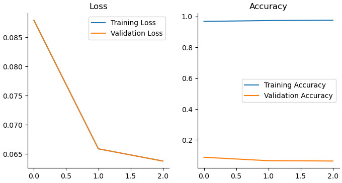
8.
val_loss, val_acc = model.evaluate(val_generator)
print(f'Validation Loss: {val_loss}, Validation Accuracy: {val_acc}')

# r :
313/313 ━━━━━━━━━━━━━━━━━━━━ 858s 3s/step - accuracy: 0.9863 - loss: 0.0379
Validation Loss: 0.037653736770153046, Validation Accuracy: 0.9869999885559082

train_generator.class_indices

# r :
{'cat': 0, 'dog': 1}


import numpy as np

val_data.loc[:, 'val_pred'] = np.argmax(val_pred, axis=1)
labels = dict((v,k) for k,v in train_generator.class_indices.items())
val_data.loc[:, 'val_pred'] = val_data.loc[:, 'val_pred'].map(labels)
val_data.head()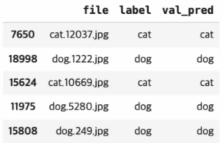
confusion_matrix 시각화
from sklearn.metrics import confusion_matrix
from sklearn.metrics import ConfusionMatrixDisplay

fig, ax = plt.subplots(figsize = (10,10))
cm = confusion_matrix(val_data['label'], val_data['val_pred'])
disp = ConfusionMatrixDisplay(counfusion_matrix=cm, display_labels=lables.values())
disp.plot(cmap=plt.cm.Blues, ax=ax)
plt.show()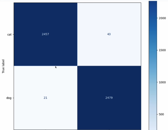

Perfect timing to be a Newbie