1. 데이터 가져오기
pip install kagglehub
import kagglehub

# Download latest version
path = kagglehub.dataset_download("ashishjangra27/face-mask-12k-images-dataset")

print("Path to dataset files:", path)

# r :
Path to dataset files: ...\versions\1


import os
import glob
import pandas as pd

path = '.../versions/1/Face Mask Dataset'

dataset = {
    'image_path': [],
    'mask_status': [],
    'where': []
}

# # 주어진 경로(path) 안의 폴더를 순회
for where in os.listdir(path):
    for status in os.listdir(os.path.join(path, where)):
    	# 주어진 경로에서 특정 패턴(*.png)에 맞는 모든 파일 경로를 찾아 리스트로 반환
        for image in glob.glob(os.path.join(path, where, status, '*.png')):
            dataset['image_path'].append(image)
            dataset['mask_status'].append(status)
            dataset['where'].append(where)

dataset = pd.DataFrame(dataset)
dataset.head()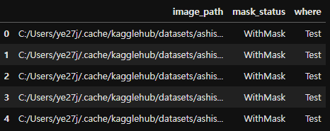
2. 간단 EDA
import seaborn as sns
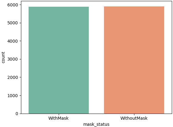
print(dataset.value_counts('mask_status'))
# r :
mask_status
WithoutMask 5909
WithMask 5883
Name: count, dtype: int64
sns.countplot(x=dataset['mask_status'], palette='Set2')
import numpy as np
import cv2 # 이미지를 읽기 위해 OpenCV를 사용

plt.figure(figsize=(8,5))

# 9개의 이미지를 무작위로 선택 및 시각화
for i in range(9):
    random = np.random.randint(0, len(dataset))

    plt.subplot(3, 3, i+1)
    # cv2.imread: 경로를 가져와 이미지를 읽음
    plt.imshow(cv2.imread(dataset['image_path'][random]))
    plt.title(dataset['mask_status'][random])
    plt.axis('off')

plt.show()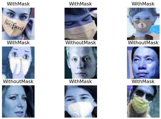
# 데이터 종류별 데이터프레임 생성
train_df = dataset[dataset['where'] == 'Train']
test_df = dataset[dataset['where'] == 'Test']
valid_df = dataset[dataset['where'] == 'Validation']

# 데이터 종류별 countplot 생성
plt.figure(figsize=(15,4))

plt.subplot(1,3,1)
sns.countplot(x = train_df['mask_status'], palette='Set2')
plt.title('Train')

plt.subplot(1,3,2)
sns.countplot(x = test_df['mask_status'], palette='Set2')
plt.title('Test')

plt.subplot(1,3,3)
sns.countplot(x = valid_df['mask_status'], palette='Set2')
plt.title('Validation')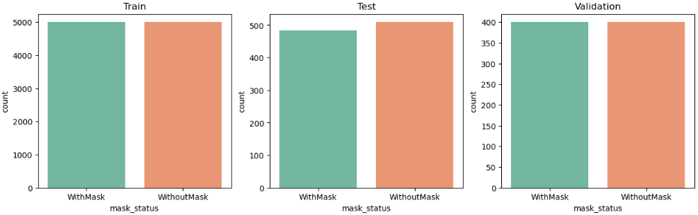
3. Train 데이터 전처리
- cv2.imread : 메모리 효율을 위해 이전에 읽은 이미지를 저장하지 않고 필요할 때마다 새로 읽음
train_df = train_df.reset_index(drop=True)

# data는 이미지 데이터와 라벨(0 또는 1)을 저장하기 위한 리스트
data = []; image_size = 50

for i in range(len(train_df)):

	# 이미지를 흑백으로 읽음 (1채널)
    # 반환되는 배열은 2차원 형태 (높이, 너비)
    # Numpy 배열(numpy.ndarray)로 이미지를 저장
    img_array = cv2.imread(train_df['image_path'][i], cv2.IMREAD_GRAYSCALE)

   	# 이미지 리사이징
    new_img_array = cv2.resize(img_array, (image_size, image_size))

    # 리스트 형태로 라벨(1 또는 0)과 함께 묶어 모델 학습에 적합하도록 구조화
    if train_df['mask_status'][i] == 'WithMask':
        data.append([new_img_array,1]) # 라벨 1 (마스크 착용)

    else:
        data.append([new_img_array, 0]) # 라벨 0 (마스크 미착)


# 첫 번째 값
data[0]

# r :
# 50x50 = 2500개의 픽셀 값
[array([[238, 238, 238, ..., 187, 194, 197],
        [237, 240, 239, ..., 177, 194, 193],
        [238, 238, 238, ..., 174, 184, 189],
        ...,
        [235, 234, 233, ..., 146, 150, 151],
        [235, 235, 233, ..., 149, 152, 152],
        [235, 234, 234, ..., 150, 151, 152]], dtype=uint8), 1]


# 리스트 형태의 데이터를 추출해서 Numpy 배열로 변환
X = np.array([item[0] for item in data])  # 이미지 배열만 추출
y = np.array([item[1] for item in data])  # 라벨만 추출

print(X.shape)  # 결과: 3차원 Numpy 배열 (데이터 개수, 50, 50)
print(y.shape)  # 결과: 1차원 Numpy 배열 (데이터 개수,)

# r :
(10000, 50, 50)
(10000,)
4. Train 데이터 시각화
# 셔플
np.random.shuffle(data)

# 행렬 형태로 정렬된 데이터를 시각화
fig, ax = plt.subplots(2,3, figsize=(10,6))

for row in range(2):
    for col in range(3):
        ax[row][col].imshow(data[row*3+col][0], cmap='gray') # 이미지
        ax[row][col].set_title(data[row*3+col][1]) # 레이블

plt.show()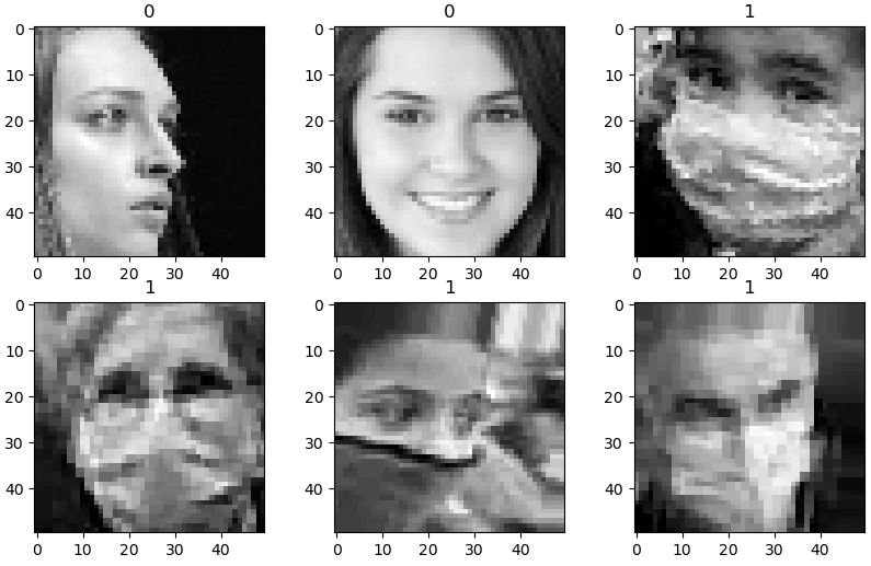
5. 입력 데이터와 라벨 분리 / Numpy 배열 변환
<배열로 바꾸는 이유>
- 머신러닝/딥러닝 모델이 데이터를 처리할 수 있는 형태로 변환하기 위해
- 모델 학습은 리스트가 아니라 Numpy 배열이나 텐서(Tensor)와 같은 고정된 형태의 데이터 구조를 요구
- 리스트 형식의 데이터를 직접 처리할 수 없으므로, 배열로 변환이 필수적
- Numpy 배열은 벡터화 연산을 지원, 대규모 데이터 연산에 적합
<데이터 준비 과정 요약>
- 데이터 수집: 데이터는 보통 리스트 형태로 관리됩니다.
- Numpy 배열로 변환: 연산 효율성과 딥러닝 프레임워크 호환성을 위해 Numpy 배열로 변환.
- 모델 입력 준비:
- 데이터 정규화 (예: 픽셀 값을 0~1 범위로 변환).
- 데이터 차원 재구성 (CNN 등 모델 입력 요구사항에 맞춤).
X=[]; y=[]

for image in data:
    X.append(image[0]) # 이미지 배열을 X 리스트에 추가
    y.append(image[1]) # 라벨 값을 y 리스트에 추가

# 리스트를 Numpy 배열로 변환
X = np.array(X) # 3차원 배열 (데이터 개수, 이미지 높이, 너비)
y = np.array(y) # 1차원 배열 (데이터 개수,)

# 데이터 정규화 (정규화 유/무에 따른 퍼포먼스 비교 필요)
X = X/255.
6. 모델 형성 / Compile - CNN 모델
<CNN 모델의 구조>
- 합성곱(Conv2D): 이미지의 특징을 추출.
- Pooling: 크기를 줄이며 중요한 정보를 유지.
- Flatten: 2D 데이터를 1D 벡터로 변환.
- Dense: 완전 연결 층으로 출력 계산.
from sklearn.model_selection import train_test_split

X_train, X_val, y_train, y_val = train_test_split(X, y, test_size=0.2, random_state=4)


from tensorflow.keras import layers, models

model = models.Sequential([

    # 32개의 (5x5) 필터를 사용
    layers.Conv2D(32, (5,5), strides=(1,1), padding='same', activation='relu',
                  input_shape=(image_size, image_size, 1)),

    # pool_size : 한 번에 2x2 영역(4개의 값)을 처리
    # strides : 윈도우가 겹치지 않고 2칸씩 이동
    layers.MaxPooling2D(pool_size=(2,2), strides=(2,2)),

    layers.Conv2D(64, (2,2), activation='relu', padding='same'),
    layers.MaxPooling2D(pool_size=(2,2), strides=(2,2)),

    # 과적합을 방지하기 위해 25%의 뉴런을 무작위로 비활성화
    layers.Dropout(0.25),

    # 2D 특성 맵을 1D 벡터로 변환해 밀집 층(Dense Layer) 연결 준비
    layers.Flatten(),
    layers.Dense(1000, activation='relu'),
    layers.Dense(1, activation='sigmoid')
])

model.summary()

# r :
Model: "sequential_1"
┏━━━━━━━━━━━━━━━━━━━━━━━━━━━━━━━━━━━━━━┳━━━━━━━━━━━━━━━━━━━━━━━━━━━━━┳━━━━━━━━━━━━━━━━━┓
┃ Layer (type)                         ┃ Output Shape                ┃         Param # ┃
┡━━━━━━━━━━━━━━━━━━━━━━━━━━━━━━━━━━━━━━╇━━━━━━━━━━━━━━━━━━━━━━━━━━━━━╇━━━━━━━━━━━━━━━━━┩
│ conv2d_3 (Conv2D)                    │ (None, 50, 50, 32)          │             832 │
├──────────────────────────────────────┼─────────────────────────────┼─────────────────┤
│ max_pooling2d_2 (MaxPooling2D)       │ (None, 25, 25, 32)          │               0 │
├──────────────────────────────────────┼─────────────────────────────┼─────────────────┤
│ conv2d_4 (Conv2D)                    │ (None, 25, 25, 64)          │           8,256 │
├──────────────────────────────────────┼─────────────────────────────┼─────────────────┤
│ max_pooling2d_3 (MaxPooling2D)       │ (None, 12, 12, 64)          │               0 │
├──────────────────────────────────────┼─────────────────────────────┼─────────────────┤
│ dropout_1 (Dropout)                  │ (None, 12, 12, 64)          │               0 │
├──────────────────────────────────────┼─────────────────────────────┼─────────────────┤
│ flatten_1 (Flatten)                  │ (None, 9216)                │               0 │
├──────────────────────────────────────┼─────────────────────────────┼─────────────────┤
│ dense_2 (Dense)                      │ (None, 1000)                │       9,217,000 │
├──────────────────────────────────────┼─────────────────────────────┼─────────────────┤
│ dense_3 (Dense)                      │ (None, 1)                   │           1,001 │
└──────────────────────────────────────┴─────────────────────────────┴─────────────────┘
 Total params: 9,227,089 (35.20 MB)
 Trainable params: 9,227,089 (35.20 MB)
 Non-trainable params: 0 (0.00 B)

 # 모델 컴파일
 model.compile(optimizer='adam', loss='binary_crossentropy', metrics=['accuracy'])
7. Train & Evaluate
X_train = X_train.reshape(-1, image_size, image_size, 1)
X_val = X_val.reshape(-1, image_size, image_size, 1)

history = model.fit(X_train, y_train, epochs=5, validation_data=(X_val, y_val))

# r :
Epoch 5/5
250/250 ━━━━━━━━━━━━━━━━━━━━ 38s 152ms/step - accuracy: 0.9699 - loss: 0.0701 - val_accuracy: 0.9740 - val_loss: 0.0743

model.evaluate(X_val, y_val)

# r :
[0.07427990436553955, 0.9739999771118164]
8. Confusion_matrix , Classification_report
from sklearn.metrics import confusion_matrix, classification_report

prediction = (model.predict(X_val) > 0.5).astype('int32')

print(classification_report(y_val, prediction))
print(confusion_matrix(y_val, prediction))

# r :
              precision    recall  f1-score   support

           0       0.99      0.96      0.98      1053
           1       0.96      0.99      0.97       947

    accuracy                           0.97      2000
   macro avg       0.97      0.97      0.97      2000
weighted avg       0.97      0.97      0.97      2000

[[1015   38]
 [  14  933]]
9. Wrong Result
wrong_result = []

for n in range(len(y_val)):
    if prediction[n] != y_val[n]:
        wrong_result.append(n)

len(wrong_result)

# r :
38


import random

samples = random.choices(wrong_result, k=6)

plt.figure(figsize=(8,4))

for i in range(6):
    plt.subplot(2,3, i+1)
    plt.imshow(X_val[samples[i]], cmap='gray')

plt.show()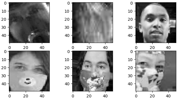

Perfect timing to be a Newbie