WINE

[v.2] Pipeline 추가

데이터 불러오기

import pandas as pd

red_url = '.../winequality-red.csv'
white_url = '.../winequality-white.csv'

red_wine = pd.read_csv(red_url, sep=';')
white_wine = pd.read_csv(white_url, sep=';')

테이블 합치기

red_wine['color'] = 1
white_wine['color'] = 0

wine = pd.concat([red_wine, white_wine])
wine.head()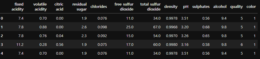

범주형 데이터 이진 변수화

wine['taste'] = [1. if grade > 5 else 0. for grade in wine['quality']]
wine.head()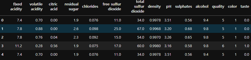

임포트

from sklearn.pipeline import Pipeline
from sklearn.preprocessing import StandardScaler
from sklearn.model_selection import train_test_split
from sklearn.tree import DecisionTreeClassifier
from sklearn.metrics import accuracy_score

Train, Test 데이터 분류

# quality는 taste와 강한 상관관계를 가질 가능성이 높은 변수. 이를 포함할 경우 모델이 단순히 quality를 사용해 taste를 예측
# 따라서 quality를 제거하여 모델이 다른 특성을 활용하도록 유도

X = wine.drop(['taste', 'quality'], axis=1)
y = wine['taste']

X_train, X_test, y_train, y_test = train_test_split(X, y, test_size=0.2, stratify=y, random_state=4)

Pipeline 생성 (StandardScaler / DecisionTreeClassifier)

• estimators는 사이킷런의 Pipeline 객체를 구성할 때 사용하는 단계들의 목록으로, 각 단계에 사용할 전처리 도구나 모델을 지정하는 역할
• Pipeline은 estimators에 지정된 순서대로 작업을 수행

estimators = [
    ('scaler', StandardScaler()),
    ('clf', DecisionTreeClassifier())]

pipe = Pipeline(estimators)
pipe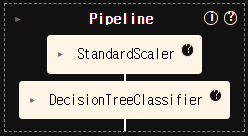

Pipeline의 파라미터 셋팅

pipe.set_params(clf__max_depth=2)
pipe.set_params(clf__random_state=4)

Pipeline 훈련

pipe.fit(X_train, y_train)

y_pred_test = pipe.predict(X_test)
accuracy_score(y_test, y_pred_test)
# 결과 : 
0.9569230769230769

Classification 모델 평가 (pipeline 적용x)

accuracy / recall / precision / f1_score / roc_auc_score / roc_curve

from sklearn.metrics import accuracy_score, recall_score, precision_score, f1_score
from sklearn.metrics import roc_auc_score, roc_curve

y_pred_tr = wine_tree.predict(X_train)
y_pred_test = wine_tree.predict(X_test)

print('accuracy_score: ', accuracy_score(y_test, y_pred_test))
print('recall_score: ', recall_score(y_test, y_pred_test))
print('precision_score: ', precision_score(y_test, y_pred_test))
print('f1_score: ', f1_score(y_test, y_pred_test))
print('roc_auc_score: ', roc_auc_score(y_test, y_pred_test))

# 결과 : 
accuracy_score:  0.7346153846153847
recall_score:  0.8578371810449574
precision_score:  0.7558886509635975
f1_score:  0.8036425725668753
roc_auc_score:  0.6899248798306549

Classification 모델 평가 그래프

import matplotlib.pyplot as plt

# predict_proba 메서드는 각 클래스에 대한 예측 확률을 반환 (각 클래스에 속할 확률) 
# 이진 분류 모델인 경우 각 샘플에 대해 두 가지 확률 값 [P(class=0), P(class=1)]을 반환
# [:, 1]은 이 확률 배열에서 두 번째 열(class=1에 대한 확률)만 선택
# ROC 곡선을 그릴 때는 양성 클래스에 대한 확률을 사용하는 것이 일반적
pred_proba = wine_tree.predict_proba(X_test)[:,1]

# fpr: 모델이 실제로는 음성 클래스(Negative)인 샘플을 양성 클래스(Positive)로 잘못 분류한 비율.
# tpr: 모델이 실제로 양성 클래스(Positive)인 샘플을 양성으로 올바르게 분류한 비율 (= recall)
# 범위: [0, 1] / TPR이 높을수록 모델이 양성을 정확히 분류하는 능력이 높음
fpr, tpr, _ = roc_curve(y_test, pred_proba)

plt.figure(figsize=(8,4))
plt.plot([0,1], [0,1], 'r')
plt.plot(fpr,tpr)
plt.grid()
plt.show()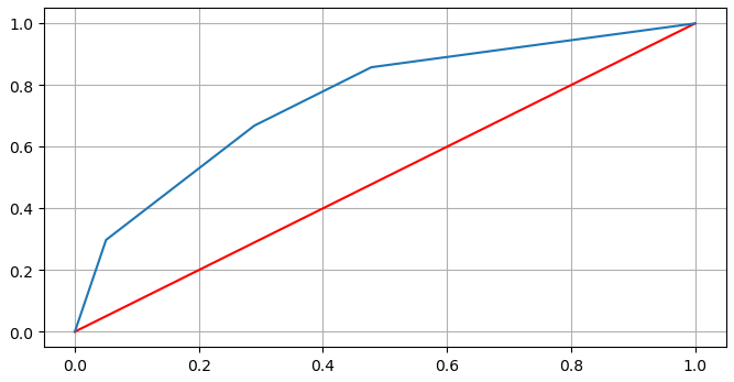

[v.3] 모델 비교 시각화 추가

데이터 불러오기 & 정리

import pandas as pd

wine_url = '.../dataset/wine.csv'
wine = pd.read_csv(wine_url, index_col=0)

wine['taste'] = [1 if grade >5 else 0 for grade in wine['quality']]

X = wine.drop(['taste', 'quality'], axis=1)
y = wine['taste']

Train, Test 데이터 분류

from sklearn.model_selection import train_test_split

X_train, X_test, y_train, y_test = train_test_split(X, y, test_size=0.2, random_state=4)

LogisticRegression - Fit / Predict / Score

• solver='liblinear'는 로지스틱 회귀(Logistic Regression) 모델에서 사용되는 매개변수
• 주요 solver 옵션
  1) liblinear: 작은 데이터셋에서 좋은 성능을 보이며, 이진 분류와 작은 데이터셋에 적합
  2) saga: 대규모 데이터셋에 적합하며, 특히 L1 규제와 L2 규제 모두에서 사용
  3) lbfgs: 기본적으로 많이 사용되는 알고리즘으로, 대규모 데이터셋에 적합
  4) newton-cg: 다중 클래스 분류에 적합하며, L2 규제와 함께 사용

from sklearn.linear_model import LogisticRegression
from sklearn.metrics import accuracy_score

lr = LogisticRegression(solver='liblinear', random_state=4)
lr.fit(X_train, y_train)

y_pred_tr = lr.predict(X_train)
y_pred_test = lr.predict(X_test)

accuracy_score(y_train, y_pred_tr), accuracy_score(y_test, y_pred_test)
# 결과 : 
(0.7463921493169136, 0.7123076923076923)

Pipeline 생성 (+Scaler) - Fit / Predict / Score

from sklearn.pipeline import Pipeline
from sklearn.preprocessing import StandardScaler

estimators = [
    ('scaler', StandardScaler()),
    ('clf', LogisticRegression(solver='liblinear', random_state=4))
]

pipe = Pipeline(estimators)
pipe.fit(X_train, y_train)

y_pred_tr = pipe.predict(X_train)
y_pred_train = pipe.predict(X_test)

accuracy_score(y_train, y_pred_tr), accuracy_score(y_test, y_pred_train)
# 결과 : 
(0.7488935924571868, 0.7169230769230769) 
# scaler 진행 전과 큰 차이는 없음 

Classification 모델 평가 그래프

models = {
    'logistic regression' : lr,
    'decision tree' : wine_tree
}

from sklearn.metrics import roc_curve
import matplotlib.pyplot as plt

plt.figure(figsize=(6,4))
plt.plot([0,1],[0,1], 'k--')

for model_name, model in models.items():
    pred = model.predict_proba(X_test)[:,1]
    fpr, tpr, _ = roc_curve(y_test, pred)
    plt.plot(fpr, tpr, label=model_name)

plt.grid()
plt.legend()
plt.show()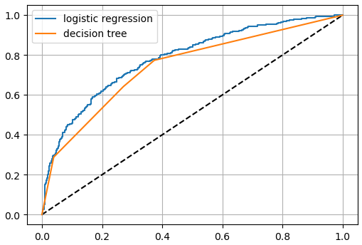

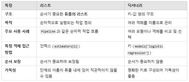
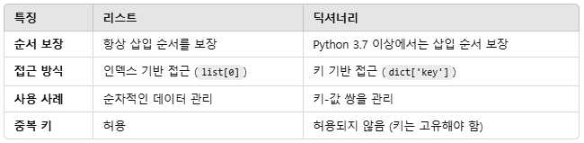
* - 리스트 (estimators 예제) / 딕셔너리 (models 예제) 차이

• 리스트 (Pipeline 사용):
  작업이 순차적으로 처리되어야 할 때 사용
  전처리 및 모델 학습이 연결된 흐름(Flow)을 나타낼 때 적합
  예: Pipeline 객체.

• 딕셔너리 (모델 비교/관리):
  여러 객체를 명확한 이름으로 관리하고 접근해야 할 때 사용
  모델의 성능 비교, 선택, 평가 등 비순차적인 작업에 적합
  예: 여러 모델 간 성능 비교를 위한 코드.
  
  

PIMA

데이터 불러오기 & 결측치 정리

PIMA_url = 'https://raw.githubusercontent.com/PinkWink/ML_tutorial/refs/heads/master/dataset/diabetes.csv'

PIMA = pd.read_csv(PIMA_url)
PIMA = PIMA.astype('float')

(PIMA==0).astype(int).sum()

zero_features = ['Glucose','BloodPressure','SkinThickness','BMI']

PIMA[zero_features] = PIMA[zero_features].replace(0, PIMA[zero_features].mean())
(PIMA[zero_features]==0).sum()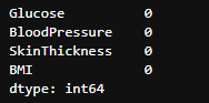

Train, Test 데이터 분류

from sklearn.model_selection import train_test_split

X = PIMA.drop('Outcome',axis=1)
y = PIMA['Outcome']

X_train, X_test, y_train, y_test = train_test_split(X,y,test_size=0.2, random_state=4, stratify=y)

Pipeline 셋팅 (StandardScaler / LogisticRegression)

from sklearn.pipeline import Pipeline
from sklearn.preprocessing import StandardScaler
from sklearn.linear_model import LogisticRegression

estimators = [
    ('scaler', StandardScaler()),
    ('clf', LogisticRegression(solver='liblinear', random_state=4))
]
pipe_lr = Pipeline(estimators)

Pipeline Train / Predict / Scoring

pipe_lr.fit(X_train, y_train)
pred = pipe_lr.predict(X_test)

from sklearn.metrics import accuracy_score, recall_score, precision_score, f1_score, confusion_matrix

print('accuracy: {:.2f}'.format(accuracy_score(y_test, pred)))
print('recall: {:.2f}'.format(recall_score(y_test, pred)))
print('precision: {:.2f}'.format(precision_score(y_test, pred)))
print('f1 score: {:.2f}'.format(f1_score(y_test, pred)))
print(confusion_matrix(y_test,pred))
# 결과 :
accuracy: 0.72
recall: 0.59
precision: 0.60
f1 score: 0.60
[[79 21]
 [22 32]]

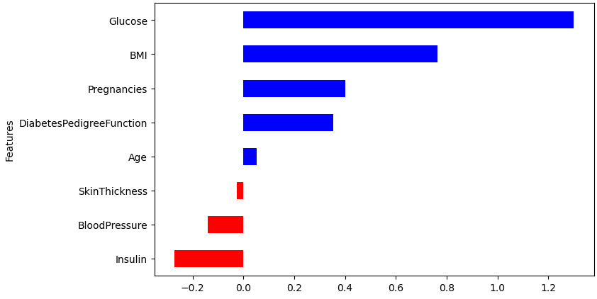
회귀 계수 (Feature별 중요도) 시각화

• 이진 분류에서는 두 클래스(class=0과 class=1)가 존재하지만, 로지스틱 회귀의 coef_는 클래스 1에 대한 계수만 저장
• coef_ 의 결과 : (계수, feature 개수)

coeff = list(pipe_lr['clf'].coef_[0])
labels = list(X_train.columns)

pipe_lr['clf'].coef_
# 결과 : 
array([[ 0.40067199,  1.30063334, -0.13956054, -0.02672671, -0.27189878,
         0.76428723,  0.35433026,  0.05208156]])

features = pd.DataFrame({'Features': labels, 'Importance': coeff})
features.sort_values(by=['Importance'], inplace=True)
features['Positive'] = features['Importance']>0

features.set_index('Features', inplace=True)

features['Importance'].plot(kind='barh', figsize=(8,5), color=features['Positive'].map({True: 'blue', False: 'red'}))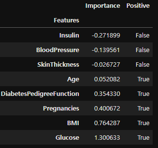

WINE

[v.4] Hyper Parameter

데이터 가져오기 & 정리

import pandas as pd

red_url = '.../data/winequality-red.csv'
white_url = '.../data/winequality-white.csv'

red_wine = pd.read_csv(red_url, sep=';')
white_wine = pd.read_csv(white_url, sep=';')

red_wine['color'] = 1
white_wine['color'] = 0

wine = pd.concat([red_wine, white_wine])

wine['taste'] = [1 if grade >5 else 0 for grade in wine['quality']]

X = wine.drop(['taste', 'quality'], axis=1)
y = wine['taste']

DecisionTreeClassifier - Train / Predict / Scoring

from sklearn.model_selection import train_test_split
from sklearn.tree import DecisionTreeClassifier
from sklearn.metrics import accuracy_score

X_train, X_test, y_train, y_test = train_test_split(X, y, test_size=0.2, random_state = 4)
wine_tree = DecisionTreeClassifier(max_depth=2, random_state=4)
wine_tree.fit(X_train, y_train)

y_pred_tr = wine_tree.predict(X_train)
y_pred_test = wine_tree.predict(X_test)

accuracy_score(y_train, y_pred_tr), accuracy_score(y_test, y_pred_test)
# 결과 : 
(0.7396574947084856, 0.7184615384615385)

Cross Validation

StratifiedKFold

• 교차 검증에서 데이터를 분할할 때 사용하는 데이터 분할 전략 객체 (cv)
• 클래스 불균형 문제를 해결하기 위해, 각 폴드에서 y 클래스 비율을 원본 데이터와 동일하게 유지
• cross_val_score, cross_validate, GridSearchCV 등에서 cv 매개변수로 사용.

cross_val_score

• 지정된 데이터 분할 전략(cv)을 사용해 주어진 모델에 대해 교차 검증을 수행하고, 테스트 점수(accuracy, f1 score etc.)만 반환
• 간단한 교차 검증 점수를 계산하는 데 적합
• 데이터 분할(split), 학습(fit), 평가(score) 과정을 모두 포함하므로 별도로 X와 y를 분할할 필요가 없음

from sklearn.model_selection import StratifiedKFold, cross_val_score

# 결정 트리 모델 생성
wine_tree_cv = DecisionTreeClassifier(max_depth=2, random_state=4)

# StratifiedKFold 객체 생성
skfold = StratifiedKFold(n_splits=5)

# 교차 검증 수행 (매개변수 순서 변경X = 모델 > X > y > cv전략)
# cv: 교차 검증 분할 전략 (skfold 객체)
cross_val_score(wine_tree_cv, X, y, cv=skfold)

# 결과 : 
array([0.55230769, 0.68846154, 0.71439569, 0.73210162, 0.75673595])

cross_validate

• 반환값은 딕셔너리 형태로, 각 폴드의 테스트 점수, 학습 점수, 학습 및 점수 계산 시간을 함께 반환

from sklearn.model_selection import StratifiedKFold, cross_validate

wine_tree_cv = DecisionTreeClassification(max_depth=2, random_state=4)

skfold = StratifiedKFold(n_splits=5)

cross_validate(wine_tree_cv, X, y, cv=skfold, return_train_score=True)
# 결과 : 
{'fit_time': array([0.01651144, 0.01403475, 0.01599216, 0.01027298, 0.010813  ]),
 'score_time': array([0.0045104 , 0.00299239, 0.00396204, 0.00199461, 0.00199318]),
 'test_score': array([0.55230769, 0.68846154, 0.71439569, 0.73210162, 0.75673595]),
 'train_score': array([0.74773908, 0.74696941, 0.74317045, 0.73509042, 0.73258946])}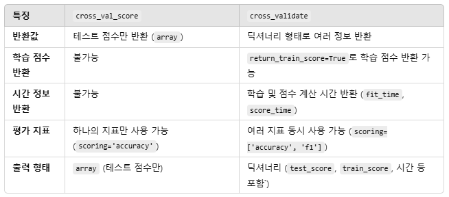

GridSearchCV

• 지정된 하이퍼파라미터 그리드에서 최적의 하이퍼파라미터 조합을 찾기 위해 교차 검증을 수행.
• 내부적으로 cross_validate을 사용하여 각 하이퍼파라미터 조합의 성능을 평가하고 최적의 조합을 선택.
• GridSearchCV는 단순히 최적의 하이퍼파라미터를 찾기 위한 도구
• GridSearchCV는 내부적으로 여러 번의 fit을 수행하여 최적의 하이퍼파라미터를 찾음
• 최적의 모델은 GridSearchCV 객체의 bestestimator에 저장
• 모델을 GridSearchCV로 튜닝한 후, 최적의 모델을 사용해 예측하거나 추가 작업을 수행하려면 fit을 호출한 결과를 사용해야 함

from sklearn.model_selection import GridSearchCV
from sklearn.tree import DecisionTreeClassifier

params = {'max_depth':[2,4,7,10]}
wine_tree = DecisionTreeClassifier(random_state=4)

grid_search = GridSearchCV(wine_tree, param_grid=params, cv=5)
grid_search.fit(X_train, y_train)

grid_search.cv_results_
# 결과 
{'mean_fit_time': array([0.0102963 , 0.01396451, 0.02435012, 0.02766619]),
 'std_fit_time': array([0.00210397, 0.00139692, 0.00164525, 0.00162327]),
 'mean_score_time': array([0.00280542, 0.00259871, 0.00239406, 0.00179524]),
 'std_score_time': array([0.00038965, 0.0008024 , 0.00048873, 0.00039077]),
 'param_max_depth': masked_array(data=[2, 4, 7, 10],
              mask=[False, False, False, False],
        fill_value='?',
             dtype=object),
 'params': [{'max_depth': 2},
  {'max_depth': 4},
  {'max_depth': 7},
  {'max_depth': 10}],
 'split0_test_score': array([0.72980769, 0.73076923, 0.73269231, 0.75480769]),
 'split1_test_score': array([0.73557692, 0.74230769, 0.74230769, 0.74903846]),
 'split2_test_score': array([0.73820982, 0.73243503, 0.73051011, 0.7545717 ]),
 'split3_test_score': array([0.74687199, 0.7574591 , 0.76419634, 0.7574591 ]),
 'split4_test_score': array([0.7333975 , 0.74013474, 0.75072185, 0.75938402]),
 'mean_test_score': array([0.73677278, 0.74062116, 0.74408566, 0.7550522 ]),
 'std_test_score': array([0.00575142, 0.0094939 , 0.01237533, 0.00349324]),
 'rank_test_score': array([4, 3, 2, 1])}

grid_search.best_estimator_
# 결과 : DecisionTreeClassifier(max_depth=10, random_state=4)

grid_search.best_score_
# 결과 : 0.7550521951580661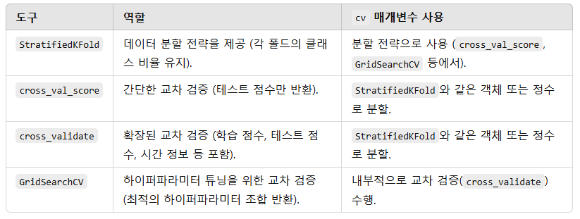

Pipeline 적용 (StandardScaler / DecisionTreeClassifier)

from sklearn.pipeline import Pipeline
from sklearn.preprocessing import StandardScaler
from sklearn.tree import DecisionTreeClassifier

estimators = [('scaler', StandardScaler()), ('clf', DecisionTreeClassifier(random_state=4))]
pipe = Pipeline(estimators)

# 하이퍼파라미터 그리드 설정
# <단계 이름>__<하이퍼파라미터 이름> 형식
param_grid = [{'clf__max_depth': [2,4,7,10]}]

# GridSearchCV 생성
grid_search = GridSearchCV(pipe, param_grid=param_grid, cv=5)
grid_search

# 교차 검증 및 모델 학습
grid_search.fit(X_train, y_train)

# 최적 점수 확인 
# best_score_는 최적의 하이퍼파라미터 조합에서 모든 폴드의 점수의 평균값 
grid_search.best_score_
# 결과 : 0.7562071518471903

[v.5] Precision & Recall

데이터 불러오기

import pandas as pd 

wine_url = '.../dataset/wine.csv'

wine = pd.read_csv(wine_url, index_col=0)
wine['taste'] = [1 if grade>5 else 0 for grade in wine['quality']]

X = wine.drop(['taste', 'quality'], axis=1)
y = wine['taste']

LogisticRegression - Train / Test / Score

from sklearn.model_selection import train_test_split
from sklearn.linear_model import LogisticRegression
from sklearn.metrics import accuracy_score

X_train, X_test, y_train, y_test = train_test_split(X, y, test_size=0.2, random_state=4)

lr = LogisticRegression(solver='liblinear', random_state=4)
lr.fit(X_train, y_train)

y_pred_tr = lr.predict(X_train)
y_pred_test = lr.predict(X_test)

accuracy_score(y_train, y_pred_tr), accuracy_score(y_test, y_pred_test)
# 결과 : 
(0.7463921493169136, 0.7123076923076923)

Precision / Recall

from sklearn.metrics import classification_report, confusion_matrix

print(classification_report(y_test, y_pred_test))
# 결과 : 
 				precision    recall  f1-score   support

           0       0.64      0.52      0.57       487
           1       0.74      0.83      0.78       813

    accuracy                           0.71      1300
   macro avg       0.69      0.67      0.68      1300
weighted avg       0.71      0.71      0.70      1300

confusion_matrix(y_test, y_pred_test)
# 결과 : 
array([[252, 235],
       [139, 674]], dtype=int64)

1. 클래스 별 recall 값 차이의 의미

• recall = 실제 양성 샘플 중에서 모델이 올바르게 양성으로 예측한 비율
• recall 값의 차이는 클래스마다 모델의 성능이 다르게 나타나는 것을 의미
• Recall 값의 차이는 클래스 1에 대해 더 잘 예측하지만, 클래스 0에 대해 상대적으로 성능이 낮음을 나타냄
• 이는 클래스 불균형, 결정 경계의 설정, 데이터 특성 등 다양한 요인에서 비롯
• 위의 방법들(가중치 조정, 임계값 변경 등)을 사용하여 Recall의 균형을 맞출 수 있음

2. 클래스별 Recall 값 분석
[클래스 0 : Recall = 0.52]

• 실제로 클래스 0인 샘플(487개) 중 52%만 올바르게 클래스 0으로 예측.
• 나머지 48%는 False Negative로 분류됨(즉, 실제로는 클래스 0인데 클래스 1로 잘못 예측).

[클래스 1 : Recall = 0.83]

• 실제로 클래스 1인 샘플(813개) 중 83%를 올바르게 클래스 1로 예측.
• 나머지 17%는 False Negative로 분류됨(즉, 실제로는 클래스 1인데 클래스 0으로 잘못 예측).

3. Recall 차이가 발생하는 이유
(1) 클래스별 데이터 분포

• 클래스 불균형: 클래스 1 (813개) 샘플이 클래스 0 (487개)보다 많음. 모델이 클래스 1에 대해 더 많은 학습 데이터를 학습했으므로, 클래스 1을 더 잘 예측할 가능성이 큼

(2) 모델의 특성

• 결정 경계의 편향: 로지스틱 회귀와 같은 선형 모델은 데이터의 분포와 결정 경계에 따라 특정 클래스에 유리한 경향을 보일 수 있음. 결과적으로 클래스 1에 대한 예측이 더 잘 수행됨

(3) 임계값(Threshold)

• 기본적으로 모델은 확률 값이 0.5 이상이면 양성(클래스 1)으로 예측. 클래스 1의 예측 확률 분포가 클래스 0보다 더 뚜렷한 경우, 클래스 1의 Recall이 더 높아질 수 있음.

(4) 데이터의 특성 차이 :

• 클래스 0과 클래스 1의 특성 분포가 매우 다를 경우, 모델이 하나의 클래스에 더 잘 적응할 가능성이 큼 (예: 클래스 1의 특성 분포가 더 선명하거나, 클래스 0의 특성 분포가 더 분산되어 있을 경우)

4. Recall 차이를 해결하려면
(1) 클래스 불균형 해결

• 가중치 조정: class_weight='balanced'를 사용해 모델이 각 클래스에 동일한 중요도를 부여하도록 설정

LogisticRegression(class_weight='balanced', solver='liblinear')

• 언더샘플링 또는 오버샘플링: 클래스 불균형을 줄이기 위해 클래스 1을 언더샘플링하거나 클래스 0을 오버샘플링.

(2) 임계값 조정: 기본적으로 0.5인 분류 임계값을 변경하여 Recall 값을 조정할 수 있습니다:

from sklearn.metrics import recall_score
y_pred_new = (model.predict_proba(X_test)[:, 1] >= 0.4).astype(int)
print(recall_score(y_test, y_pred_new, pos_label=0))  # 클래스 0의 Recall 계산
print(recall_score(y_test, y_pred_new, pos_label=1))  # 클래스 1의 Recall 계산

(3) 모델 개선

• 다른 분류 모델(예: RandomForestClassifier, XGBoost)을 사용하여 데이터의 비선형 관계를 학습.
• 모델 튜닝을 통해 성능 개선.

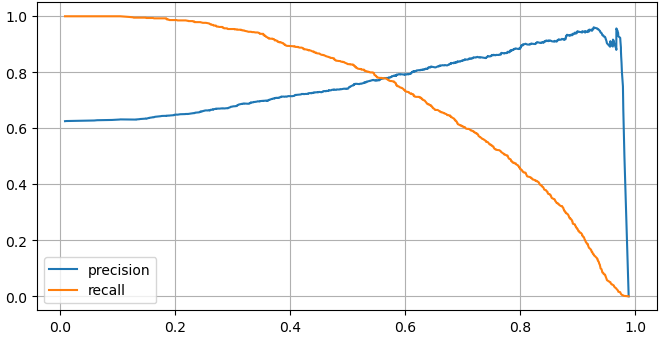
Precision / Recall 시각화

import matplotlib.pyplot as plt
from sklearn.metrics import precision_recall_curve

plt.figure(figsize=(8,4))

# predict_proba는 각 샘플이 각 클래스에 속할 확률을 반환
# [:, 1]은 두 번째 열(클래스 1의 확률)만 추출
pred = lr.predict_proba(X_test)[:,1]
precision, recall, threshold = precision_recall_curve(y_test, pred)

# thresholds는 각 경계값에서의 precision과 recall을 계산하므로, 배열 길이를 맞추기 위해 precision[:-1]와 recall[:-1]를 사용
# 가장 낮은 확률값과 가장 높은 확률값의 외부 경계를 포함하지 않음
plt.plot(threshold, precision[:-1], label='precision')
plt.plot(threshold, recall[:-1], label='recall')
plt.grid()
plt.legend()
plt.show()

# 참고 
pred_proba = lr.predict_proba(X_test)
pred_proba
# 결과 : 
array([[0.08832224, 0.91167776],
       [0.43973537, 0.56026463],
       [0.11991766, 0.88008234],
       ...,
       [0.23679924, 0.76320076],
       [0.06032141, 0.93967859],
       [0.05777677, 0.94222323]])

결과 분석 (참고)

import numpy as np

np.concatenate([lr.predict_proba(X_test), y_pred_test.reshape(-1,1)], axis=1)
# 결과 :
array([[0.08832224, 0.91167776, 1.        ],
       [0.43973537, 0.56026463, 1.        ],
       [0.11991766, 0.88008234, 1.        ],
       ...,
       [0.23679924, 0.76320076, 1.        ],
       [0.06032141, 0.93967859, 1.        ],
       [0.05777677, 0.94222323, 1.        ]])
       
np.concatenate([lr.predict_proba(X_test), y_test.values.reshape(-1,1)], axis=1)
# 결과 : 
array([[0.08832224, 0.91167776, 1.        ],
       [0.43973537, 0.56026463, 0.        ],
       [0.11991766, 0.88008234, 0.        ],
       ...,
       [0.23679924, 0.76320076, 0.        ],
       [0.06032141, 0.93967859, 1.        ],
       [0.05777677, 0.94222323, 1.        ]])

Binarizer

• 특성 변환 도구로, 지정한 임계값(threshold)을 기준으로 데이터를 이진화
• 즉, 입력 값이 임계값보다 크면 1로, 작거나 같으면 0으로 변환
• threshold를 기본값(0.5)에서 0.6으로 조정한 결과 (precision > recall구역)

from sklearn.preprocessing import Binarizer

biz = Binarizer(threshold=0.6).fit(pred_proba)
pred_bin = biz.transform(pred_proba)[:,1]
pred_bin[:5]
# 결과 : 
array([1., 0., 1., 1., 0.])

print(classification_report(y_test, pred_bin))
# 결과 : 
              precision    recall  f1-score   support

           0       0.61      0.68      0.64       487
           1       0.79      0.74      0.76       813

    accuracy                           0.71      1300
   macro avg       0.70      0.71      0.70      1300
weighted avg       0.72      0.71      0.72      1300

confusion_matrix(y_test, pred_bin)
# 결과 : 
array([[331, 156],
       [215, 598]], dtype=int64)