1. 데이터 불균형 문제 해결 - 샘플링
1.1 샘플링
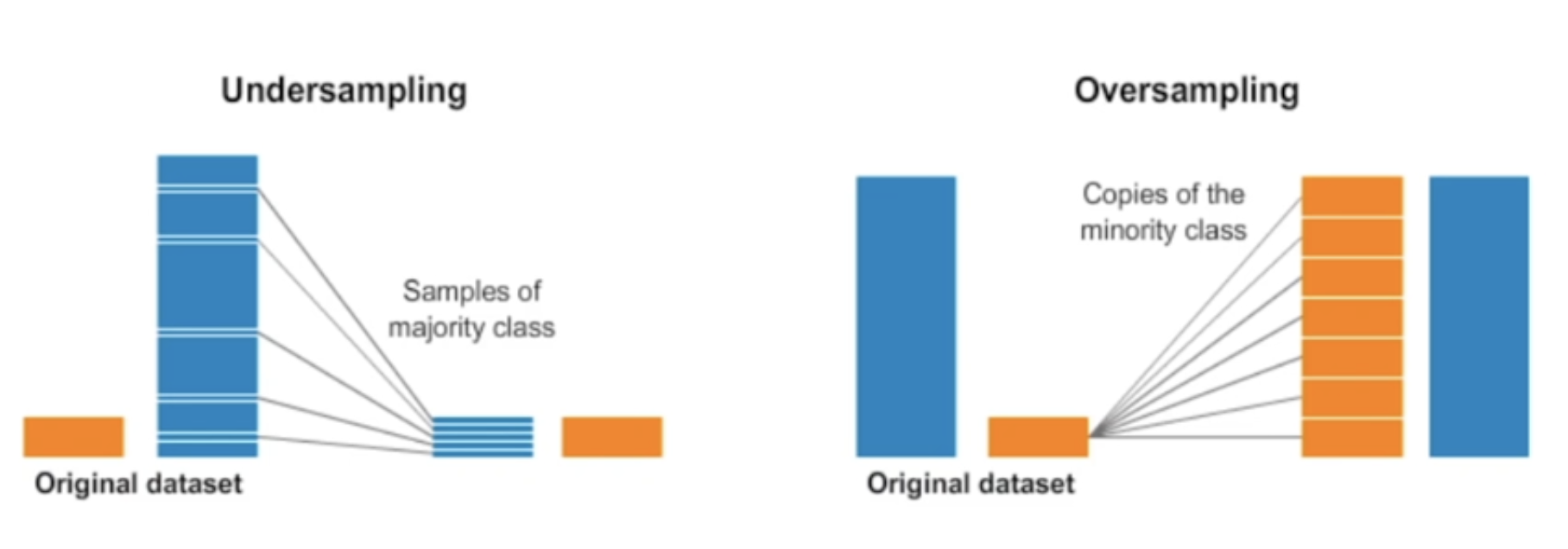
오버샘플링(Oversampling)은 소수 클래스의 샘플 수를 증가시켜서 데이터셋 클래스의 균형을 조절하는 방법이다.
- 이를 통해서 소수 클래스의 정보를 더 많이 활용하게 되어서 모델이 더 정확하게 학습되거나 더욱 다양하게 데이터를 활용할 수 있는 장점이 있다.
언더샘플링(Undersampling)은 반대로 다수 클래스의 샘플 수를 감소시켜서 데이터셋 클래스의 균형을 조절하는 방법이다.
만약 데이터 셋의 양이 충분하지 않은데 언더샘플링을 하게 된다면 비율의 문제를 떠나서 표본수 자체가 적기 때문에 모집단을 대표하는데 적합하지 않을 수 있다.
오버샘플링의 문제는 어떻게 없던 데이터를 좋은 퀄리티의 데이터로 생성하느냐다. 단순하게 복사 붙여넣기로 추가한다면 질적으로 매우 떨어질 수 있다.
1.2 데이터 불균형 문제 해결론
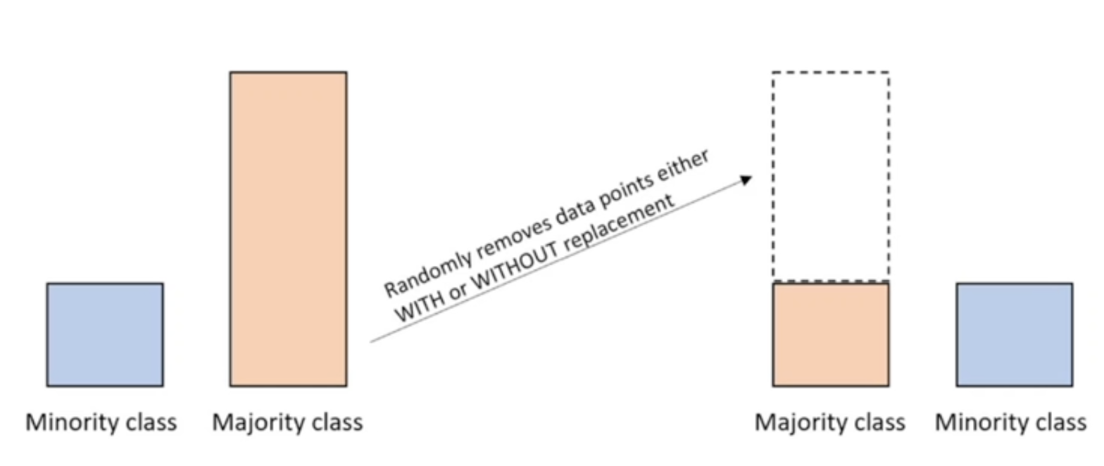
언더샘플링을 활용하여 다수의 클래스 중에 랜덤하게 값을 뽑아서 삭제하여 소수 클래스의 비율과 맞추는 방법이다.
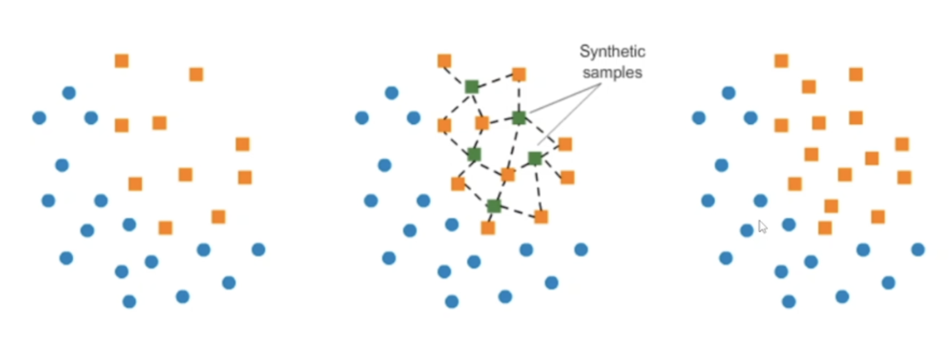
오버샘플링은 SMOTE 방법을 활용하여
왼쪽 그래프에서 소수 주황색 데이터들 중에서 특정 벡터와 가장 가까운 이웃간 사이의 차이를 계산해서 그 차이의 0과 1 사이의 난수를 곱해서 가운데 그래프처럼 새로운 초록색 타겟 벡터를 추가하게 된다.
단순히 소수 주황색 데이터를 복사 붙여넣기 해서 동일한 값들을 계속 수만 채우는게 아닌 개별 데이터마다 근처에 있는 값들을 활용해서 유사하지만 같은 값이 아닌 새로운 초록색 데이터를 생성해내는 방법이다.
1.3 샘플링 라이브러리

Imbalanced learn 라이브러리를 활용하여 샘플링으로 데이터 불균형 문제를 해결할 수 있다.
2. 데이터 불군형 문제 해결하기
# Imbalnced-learn 라이브러리 설치
!pip install imbalanced-learn
2.1 샘플링 전과 후 비교 출력
def print_result(y, y_resampled):
	print("Before")
    print("클래스 0 샘플 수:", sum(y == 0))
    print("클래스 1 샘플 수:", sum(y == 1))

    print()
    print("After")
    print("클래스 0 샘플 수:", sum(y_resampled == 0))
    print("클래스 1 샘플 수:", sum(y_resampled == 1))
# sum(y == 0) 계산 방식 import numpy as np arr = np.array([0, 0, 1, 1, 0]) arr == 0 # array([ True, True, False, False, True]) sum(arr == 0) # 3
2.2 샘플링 전과 후 비교 시각화
import matplotlib.pyplot as plt

def visualize_sampling(X, y, X_resampled, y_resampled, method_name):
    plt.figure(figsize=(10, 5))

    plt.subplot(1, 2, 1)
    # Class 0
    plt.scatter(X[y==0][:, 0], X[y==0][:, 1], label='Class 0', alpha=0.5)
    # Class 1
    plt.scatter(X[y==1][:, 0], X[y==1][:, 1], label='Class 1', alpha=0.5)
    plt.title('Original Data Distribution')
    plt.legend()

    plt.subplot(1, 2, 2)
    # Class 0
    plt.scatter(X_resampled[y_resampled==0][:, 0], X_resampled[y_resampled==0][:, 1], label='Class 0', alpha=0.5)
    # Class 1
    plt.scatter(X_resampled[y_resampled==1][:, 0], X_resampled[y_resampled==1][:, 1], label='Class 1', alpha=0.5)
    plt.title('Data Distribution After {method_name}')
    plt.legend()

    plt.tight_layout()
    plt.show()
matrix = np.array([ [1, 2], [2, 3], [3, 4], [4, 5], [5, 6] ]) print(matrix[arr==0]) print(matrix[arr==0][:, 0]) print(matrix[arr==0][:, 1]) # 결과값: # [[1 2] # [2 3] # [5 6]] # [1 2 5] # [2 3 6]
2.3 Oversampling
# 오버샘플링 이전 예제 데이터 생성
from sklearn.datasets import make_classification
from imblearn.over_sampling import SMOTE

# 가상의 데이터 생성
X, y = make_classification(
	n_classes=2, class_sep=2, weights=[0.1, 0.9], flip_y=0,
    n_clusters_per_class=1, n_samples=1000, random_state=10)
class_sep 매개변수:
- 값이 크면 클래스 간 데이터 포인트들이 서로 멀어지는
- 값이 작으면 클래스 간 데이터 포인트들이 서로 가까워지는
# SMOTE 오버샘플링 적용
smote = SMOTE(random_state=42)
X_resampled, y_resampled = smote.filt_resample(X, y)print_result(y, y_resampled)
# 결과값:
# Before
# 클래스 0 샘플 수: 100
# 클래스 1 샘플 수: 900
# After
# 클래스 0 샘플 수: 900
# 클래스 1 샘플 수: 900# 산점도 확인
visualize_sampling(X, y, X_resampled, y_resampled, 'SMOTE')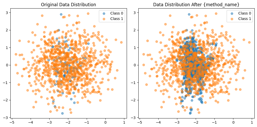
1.2 Undersampling
# 언더샘플링 이전 예제 데이터 생성
from imblearn.under_sampling import RandomUnderSampler

# 가상의 데이터 생성
X, y = make_classification(
	n_classes=2, class_sep=2, weights=[0.1, 0.9], flip_y=0,
    n_clusters_per_class=1, n_samples=1000, random_state=10)
# 랜덤 언더샘플링 적용
rus = RandomUnderSampler(random_state=42)
X_resampled, y_resampled = rus.fit_resample(X, y)print_result(ym y_resampled)
# 결과값:
# Before
# 클래스 0 샘플 수: 100
# 클래스 1 샘플 수: 900
# After
# 클래스 0 샘플 수: 100
# 클래스 1 샘플 수: 100# 산점도 확인
visualize_sampling(X, y, X_resampled, y_resampled, 'Random Under Sampling')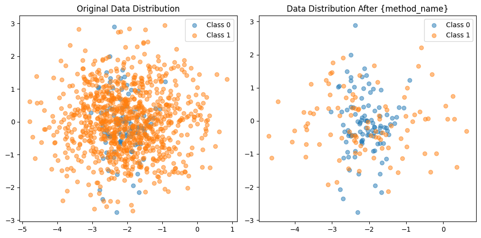

거북선통통통통