[2021 NIPS] Focal Attention for Long-Range Interactions in Vision Transformers
Paper Review
Microsoft Research, Microsoft Cloud + AI 공동 연구팀에서 NIPS 2021에 발표한 논문으로 fine-graiend local attention과 coarse-grained global attention을 한 번에 수행하는 attention 메커니즘인 focal attention을 제안한다.
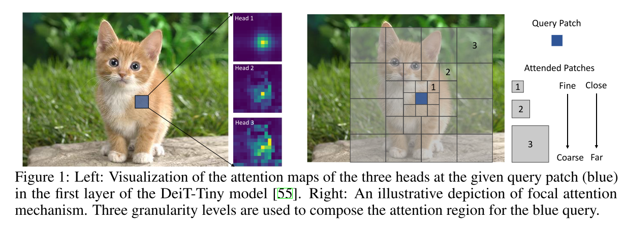
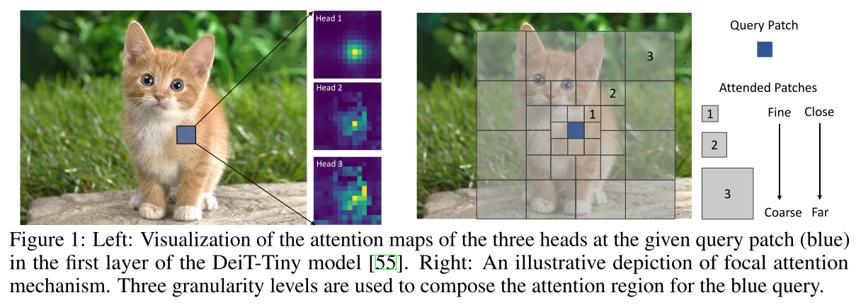
이 메커니즘에서는 각 token이 가장 가깝게 둘러싼 token들은 fine granularity에서, 멀리 있는 token들은 coarse granularity에서 attend하여 단/장 범위의 시각적 의존성을 모두 capture할 수 있게 된다.
github: https://github.com/microsoft/Focal-Transformer
Chap GPT 요약:
Vision Transformer는 최근 이미지 분류 및 객체 감지 등의 문제에서 좋은 성능을 보이는 딥러닝 모델입니다. 하지만 이 모델은 이미지의 장거리 관계를 모델링하기 어렵다는 한계가 있었습니다. 이를 해결하기 위해 "Focal Attention for Long-Range Interactions in Vision Transformers" 논문에서는 새로운 어텐션 메커니즘인 "FOCAL Attention"을 제안합니다.
FOCAL Attention은 입력 이미지를 패치 단위로 나눈 후, 각 패치에 대한 어텐션 매커니즘을 계산합니다. 이후 이 패치 어텐션의 결과를 바탕으로 전역 정보를 모델링하는 FOCAL 어텐션을 사용하여 장거리 관계를 모델링합니다. 이렇게 함으로써 패치 어텐션의 결과를 활용하여 이미지의 장거리 관계를 더 잘 모델링할 수 있게 됩니다.
실험 결과, FOCAL Attention은 비전 트랜스포머 모델에서 전반적인 성능을 향상시키는 효과를 보이며, 특히 장거리 관계를 고려할 때 더욱 효과적입니다. 이를 통해 FOCAL Attention은 이미지 분류 및 객체 감지 등의 문제에서 비전 트랜스포머 모델의 성능을 높이는 데 유용하다는 것이 보여졌습니다.
3. Method
3.1. Model Architecture
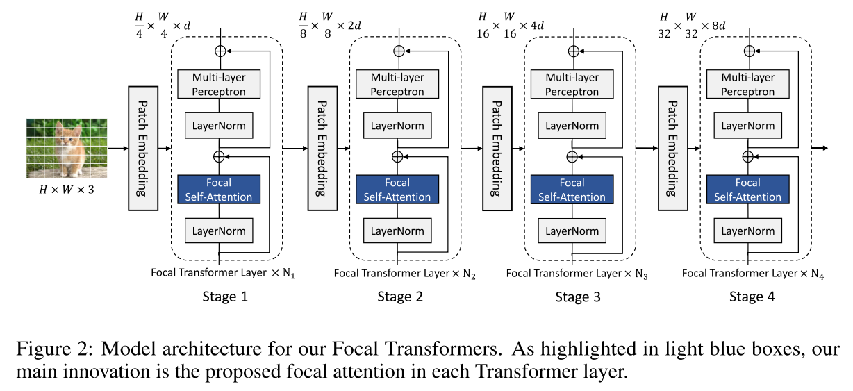
patch partioning: H x W x 3 -> (4 x 4 tokens) -> H/4 x W/4 x 3
patch embedding layer: conv (k size = stride = 4) -> project these patches to dimension d
stages: 4개, 2배씩 downsampling 되고, 그때마다 2배씩 feature dimension 키움
classification task에서는 마지막 stage의 output을 avegae해서 classfication layer로 보냄
object detection task에서는 3번째나 4번째 stage에서 특정 object head로 연결
Standard self-attention은 fine-grain에서 short and long-rage interaction을 모두 잡을 수 있는 장점이 있지만, high resolution에서 resolution의 제곱의 복잡도때문에 computational cost가 커짐
3.2. Token-wise focal attention
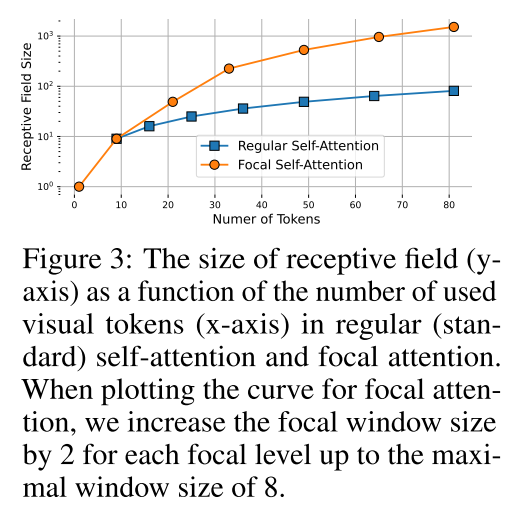
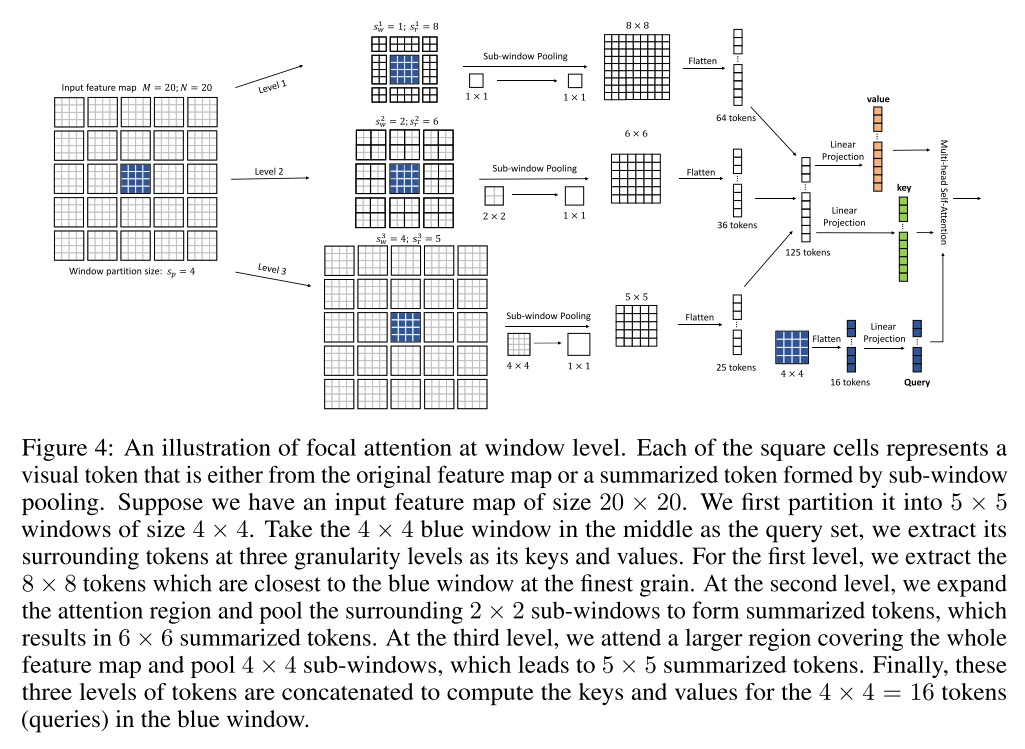
Focal attention은 Transformer layer가 고해상도 입력 이미지를 encoding 하기에도 적합하도록 만들어준다. 모든 token을 fine-grain에서 사용하는 대신 국소적으로 fine-grained token을 사용하고 sub-window pooling을 통해 생성된 coarse-grained token들을 사용한다. 그래서 기존 self-attention 보다 적은 cost로 같은 이미지 영역을 커버한다.
그림은 token 숫자에 따른 receptive field가 더 큰 것을 확인할 수 있다. 거리에 따라 둘러쌓인 query의 세분성을 감소시킴으로써 더 큰 receptive filed를 가질 수 있다.
3.2.1. Window-wise focal attention (핵심)
Terms
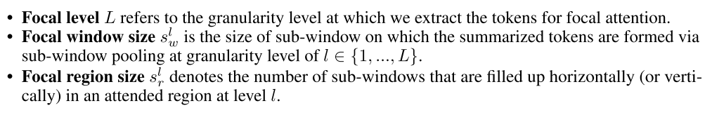
Sub-window pooling

input feature map:
sub-window: ()
linear layer: , pooling the sub-windows spatially
pooled feature maps:
focal level 에서 에 해당하는 크기의 sub-window의 grid로 split하고 sub-window들을 sptially pool하기 위한 projection layer 사용
그림을 보면 더 이해가 쉬운데 가운데 4x4 크기의 query 기준으로 각 level에 따라
다른 크기의 sub-window를 grid로 pooling한다고 보면 됨
그림과 다르게 식에선 surrounding token을 고려하지 않고 sub-window 크기로 전체 featuremap을 다 grid로 해서 pooling으로 넘기는 듯 하다
Attention computing
fisrt level의 query와 모든 level의 key, value를 linear projection layer로 아래와 같이 계산함.

focal self-attention을 수행하기 위해, 먼저 query들을 둘러쌓인 token들을 추출해야되는데 (그림에선 poolin할 때 하는 것처럼 되어있음)
앞서 언급한 것처럼 window partion 크기로 window partion 안의 token들은 같은 set of surroundings을 가짐
i-th widnow 안의 query 에 대해 모든 level에서 크기의 key와 value를 추출한다. 그림에서 첫 level에서 query 기준으로 둘러쌓인 set을 기준으로 8x8, 6x6, 5x5 pooled feature map을 추출하고 그걸 64, 36, 25 tokens (fine-grained -> coarse-grained)으로 만들어 key와 value로 만드는 부분
strict 버전의 focal attention에서는 서로 다른 level에서 overlapped region은 exclude한다

는 learnable relative position bias.
Swin Transformer와 유사하게, first level에서는 크기로 수평/수직 범위를 양쪽으로 고려해서 로 파라미터화함
다른 focal level에서는 query들의 서로 다른 granularity를 고려해서 window 안의 모든 query를 동일하게 대하는데, 각 pooled token (그림 8x8, 6x6 ,..)들과 query window 사이의 relative bias를 표현하는 를 사용함
각 window에 대한 focal attention은 서로 독립적으로 이루어져서 (3) 식이 parallel하게 진행된다 (그림에선 다 합친 token으로 하는 것으로 보이지만, )
input feature map 전체에 대한 attention score를 얻고 나면 LayerNorm, MLP block으로 보내게 된다
3.2.2. Complexity analysis
input feature map:
sub-windows at focal level 1:
각 sub-window에 대해서 아래 (1) 식의 pooling operation의 복잡도는 이고 이걸 aggregate하는 데에는 , 모든 focal level에 대해선 가 됨.

attention compuation은 query window 에 대한 attention compuation은 가 되고 모든 input feature map 전체에 대해선
3.3. Model configuration
Swin Transformer의 Tiny, Small, Base의 디자인을 따른다. 모델들은 224x224 이미지를 입력으로 받고 Swin Trasformer들과 비교할 수 있도록 window partition size ()는 7까지 설정했다
fine-grained local attention ()이랑 coarse-grained global attention () 두 개를 사용한 focal attention layer를 사용 (테이블의 Transfblock의 각 level)
마지막 stage 빼고는 (level 0) window partition size () 7에 대해서 focal region size ()를 13으로 설정했는데, 각 window partition에 대해서 3 tokens을 확장하는 걸 의미한다. (위, 아래로 3 token 씩 7 + 3 + 3 -> 13)
★★★★★
이해를 돕기 위한 예시
stage 2.
input feature map: 28 x 28
window partitioning: 7 x 7
-> 7 x 7 사이즈의 partitioned window가 4 x 4 개
0 level의 focal window size, focal region size은 1, 13이라는 뜻은 7 x 7 query를 둘러쌓은 3겹의 1x1 local focal window를 선택해서 1 x 1 크기로 pooling하면 focal region 크기 13 (7+3+3) x 13 (7+3+3)의 pooled feature map이 나온다는 뜻
1 level의 focal window size, focal region size은 7, 5이라는 뜻은 7 x 7 query를 둘러쌓은 2겹의 7x7 local focal window를 선택해서 7 x 7크기로 pooling하면 focal region 크기 5 (1+2+2) x 5 (1+2+2)의 pooled feature map이 나온다는 뜻 (padding을 주는 것인지..)
마지막 stage는 level 0의 focal region size를 7로 설정하여 feature map 전체를 cover하도록 하였다.
coarse-grained global attention ()의 경우에는 focal window size를 window partition size와 같은 7로 설정했고 focal region size를 {7, 5, 3, 1}로 점점 줄였다
patch embedding layer에 대해선, spatial reduction ratio 는 {4, 2, 2, 2)로 설정됨
다만, Focal-Base는 Focal-Tiny와 Focal-Small에 비해 더 높은 hidden dimension 을 가진다.
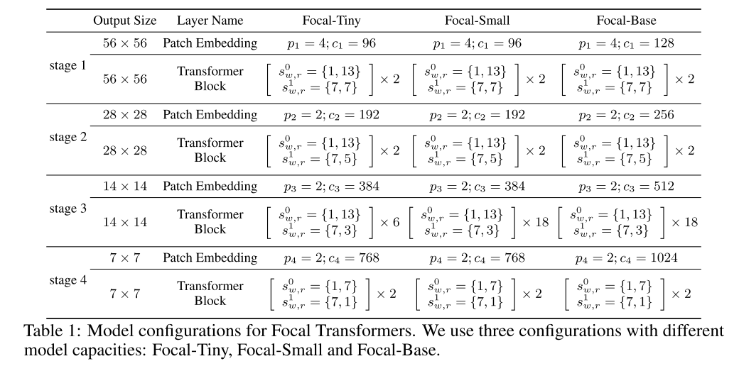
4. Experiments
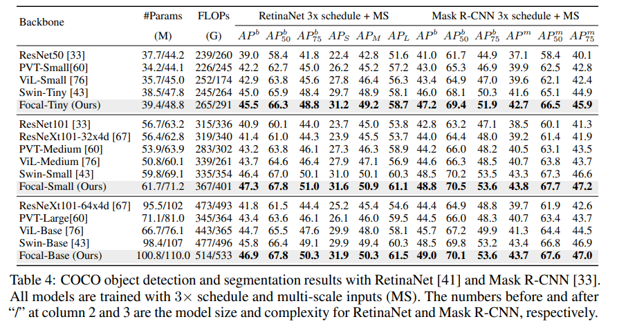
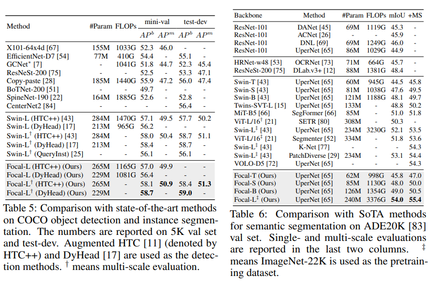
Focal-Large 모델이 classification, object detection, segmentation에서 이전 SOTA라고 볼 수 있는 Swin의 성능을 이기면서 SOTA를 찍었으나 paramter 수도 같이 증가한 부분이 조금 애매하다
Segmemtation에서는 UperNet의 방법을 썼는데, Transformer Encoder block의 representation ability가 좋다면 SegFormer을 따르면 더 효과적이었을 것 같음
같은 parameter수 대비 SegFormer보다 성능이 안 나오네.. SegFormer를 저 정도로 parameter를 키운다면..? 그냥 SegFormer의 Efficient Self-attention이 더 효과적인 게 될 수도
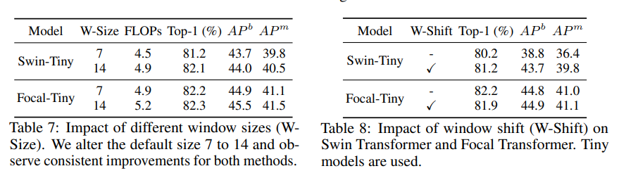
window shift 성능저하 일으켜 불필요해
Contributions of local and global interactions & Model capacity against model depth focal attention (★)
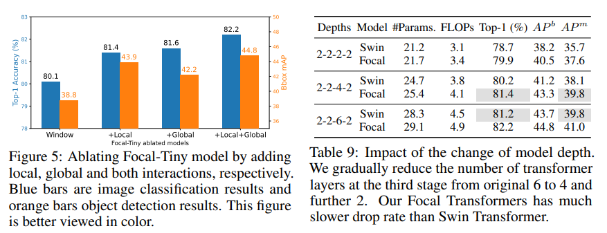
기존 전체 window에 대해서 self-attention이랑 비교했을 때, local, global 따로 하는 것도 도움이 되고 같이 했을 떈 훨씬 성능이 개선이 되더라..
그러므로 focal attention이 기존 self-attention보다 어떤 면으로 보나 낫다?
capacity로 비교했을 때도 Parameter수가 더 적은 2-2-4-2 Focal이 2-2-6-2 랑 같은 성능!
5. Conclusion
이 논문은 단/장 거리의 text (query를 둘러쌓은 세밀한 단위의 local 정보와 coarse한 단위의 global 정보)를 모두 효과적으로 capture할 수 있는 focal attention을 소개하여 Sota를 달성했고, 넓은 범위의 vision task에서 general하게 사용할 수 있는 backbone을 소개하였다.
다만, compuational cost는 한계로 남아있다.
Comments
Trasformer Block
query에 대해서 naive하게 일정한 크기의 window로 모든 key, value를 추출해서 하는 것보다 넓게 볼 건 보고 세밀하게 볼 건 세밀하게 보는 걸 구현한 focal attention으로 구현했는데, 실제로도 효과적인 걸 보였으니 기본보단 이걸 쓰는 게 낫다.
Segmentation
TopFormer (CVPR 2022)에서 neck부분에서만 Transformer Block을 사용해서 크게 computational cost를 줄였는데, SegFormer의 efficient self-attention이나 이 논문의 focal attention으로 대체하면 성능이 더 오를 것 같다.. neck 부분이면 거의 texture 다 빼고 낮은 resolution의 semantic 정보를 학습하는 feature map이라 focal attention 불필요할 수도..있나