DDPM-(5): Diffusion 한 눈에 이해하기

YEOM JINSEOP·2023년 12월 17일

Generative Model

목록 보기

4/4

참고1: Annotated Diffusion
참고2: Diffusion Model 과 DDPM 수식 유도 과정

이론

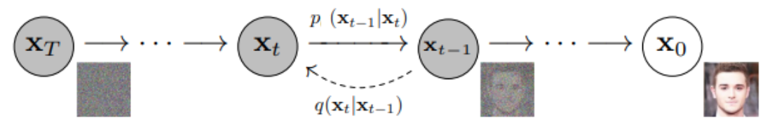
Diffusion이 풀고자 하는 문제는
forward process와 reverse process를 거친 'output 이미지 $\bold{x_0}$ '를 샘플링하는 확률분포 $\bold{p(x_0)}$ 를
'input 이미지 $\bold{x_0}$ '를 샘플링하는 확률 분포 $\bold{q(x_0)}$ 와 유사하게 만드는 것이다.
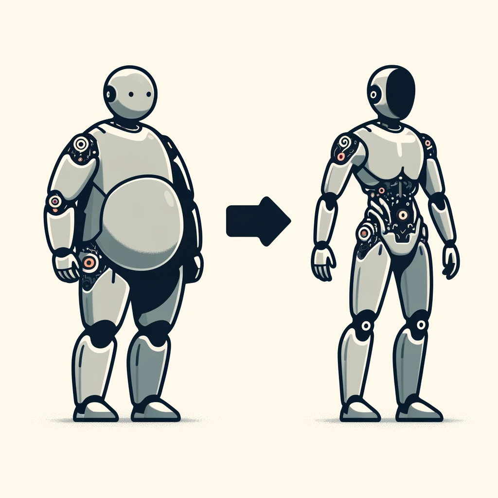
직관적으로 생각해보면,
Forward process를 거치면서
input 이미지 $\bold{x_0}$ 에 노이즈를 time step $\bold{T}$ 만큼 추가해 pure Gaussian noise $\bold{x_T}$ 를 얻은 후에
$\bold{q(x_t|x_{t-1})=N(x_t;\sqrt{1-\beta_t}x_{t-1}, \beta_tI)}$
$\\$
다시 Reverse process를 거치면서
$\bold{p(x_{t-1}|x_t)}$ 를 이용해 Gaussian noise $\bold{x_T}$ 로부터 $\bold{x_0}$ 를 샘플링하면 될 것이다.

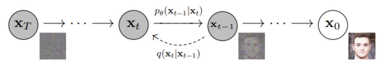
하지만, 우리는 확률 분포 $\bold{p}$ 를 알지 못한다.
그래서 우리는 신경망을 이용해서, 확률분포 $\bold{p}$ 를 가장 잘 모델링하는, 확률분포 $\bold{p_{\theta}}$ 를 예측하고 학습한다.
즉, 우리가 예측하는 확률분포 $\bold{p_{\theta}}$ 에서 $\bold{x_0}$ 가 샘플링될 확률이 가장 높게
= Likelihood $\bold{p_{\theta}(x_0)}$ 가 가장 크도록
= 확률분포 $\bold{p_{\theta}}$ 가 $\bold{p}$ 에 가까워지도록
신경망을 훈련하면 되겠다!
$\bold{p_{\theta}(x_0)}$ 를 최대화 하는 parameter $\theta$ 는
$log\bold{p_{\theta}(x_0)}$ 를 최대화 하는 parameter $\theta$ 와 동일하다. 수식 전개의 편리함을 위해 $log\bold{p_{\theta}(x_0)}$ 를 사용한다.
$\\$
$log\bold{p_{\theta}(x_0)}$ 를 최대화 하는 수식을 전개하다보면,
$\bold{p(x_{t-1}|x_t, x_0)}$ 과 $\bold{p_{\theta}(x_{t-1}|x_t)}$ 간의 KL-Divergence를 최소화하는 식으로 전개된다.
$\\$
이는 두 분포 간의 평균의 차이를 최소화하는 식으로 전개되며,
$\bold{||\tilde{\mu_t}{(x_t, x_0)} - \mu_{\theta}(x_t, t)||^2}$
$\\$
위 식을 수학적인 트릭(Reparameterization trick)을 사용하면 (=수식적으로 전개하다보면)
결국 time step $t$ 시점에 실제로 추가된 노이즈 $\epsilon$ 과 신경망이 예측한 $t$ 시점의 노이즈 $\epsilon_{\theta}$ 간의 차이를 최소화하는 식으로 전개된다.
$||\epsilon - \epsilon_{\theta}(\bold{x_t, t})||^2 = ||\epsilon - \epsilon_{\theta}(\bold{\sqrt{\bar{\alpha_t}}x_0 + \sqrt{1-\bar{\alpha_t}}\epsilon,t})||^2$

정리하면, 확률분포 $\bold{p_{\theta}}$ 가 $\bold{p}$ 에 가까워지도록 신경망을 학습시키기 위해선
확률분포 $\bold{p_{\theta}}$ 와 확률분포 $\bold{p}$ 간의 loss 함수를 정의해야 한다.
- Diffusion에서는 확률분포 $\bold{p}$ 와 확률분포 $\bold{p_{\theta}}$ 가 정규 분포(gaussian distribution)을 따른다고 설정한다.
  정규분포는 두 가지 정보, 평균( $\mu$ )과 분산( $\sigma$ )으로 표현된다.
- 그렇다면, "확률분포 $\bold{p}$ 의 평균( $\bold{\tilde{\mu}}$ ), 분산"과
  "확률 분포 $\bold{p_{\theta}}$ 의 평균( $\bold{\mu_{\theta}}$ ), 분산"의 차이를 줄이는 loss 함수를 만들면 되겠다.
- DDPM에서는 분산은 고정된(fixed) 값으로 두고 평균의 차이를 줄이는 방식을 사용했다.
  이후에 분산까지 학습하는 연구가 나오긴 했으나, 지금은 DDPM을 기준으로 생각하자.
- 수학적인 트릭(Reparameterization trick)을 사용하면
  (=수식적으로 전개하다보면)
  "확률분포 $\bold{p}$ 의 평균( $\bold{\tilde{\mu}}$ )"과, "확률 분포 $\bold{p_{\theta}}$ 의 평균( $\bold{\mu_{\theta}}$ )"의 차이를 줄이는 loss function 수식을
  "이미지에 실제로 추가된 노이즈( $\epsilon$ )"과 "신경망이 예측한 노이즈( $\epsilon_{\theta}$ )"의 차이를 줄이는 loss function 수식으로 전개가 가능하다.
- 따라서, 신경망은 이미지에 추가된 노이즈를 예측하도록 설계한다.

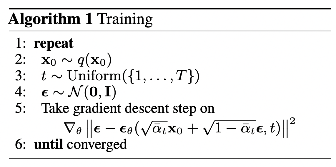
Training 과정에서,
실제 신경망 학습이 어떻게 진행되는지 알고리즘을 정리해보면,

1) real unknown and possibly complex data distribution $\bold{q(x_0)}$ 로부터
random sample $\bold{x_0}$ 를 뽑는다.
2) $\bold{1}$ 과 $\bold{T}$ 사이의 random한 noise level (= random time step) $\bold{t}$ 를 뽑는다.
3) Gaussian distribution으로부터 noise $\bold{\epsilon}$ 을 뽑는다.
4) input image $\bold{x_0}$ 에 noise level $\bold{t}$ 만큼 노이즈를 추가한다.
(known scheldue $\beta_t$ 만큼 noise가 추가된다.)
5) 신경망은 노이징된 image $\bold{x_t}$ 에 추가된 noise를 예측하도록 training한다.
(실제 구현에선, 데이터의 여러 batch들에서 위 과정이 이루어진다. 그리고 stochastic gradient descent를 사용해 신경망을 최적화한다.)

Inference 과정에서는,
$\bold{p_\theta}$ 를 학습한 신경망으로 pure Gaussian noise $\bold{x_T}$ 로부터 denoising해서 output image $\bold{x_0}$ 를 sampling한다.

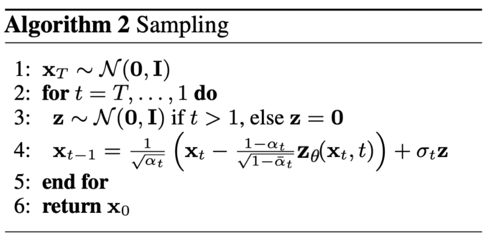
1) time step $T$ 의 pure noise에서 Gaussian distribution을 sampling한다.
$\bold{x_t} \sim N(\bold{0,I})$
2) Denoising
time step $\bold{T}$ 부터 0까지, 신경망을 사용해서, 신경망이 학습한 conditional probability를 이용해 점진적으로 denoise한다.
mean을 reparameterization하여 만든 우리의 noise predictor를 이용해서,
우리는 조금 더 denoised 된 image $\bold{x_{t−1}}$ 을 얻을 수 있다.
이 과정을 통해 real data distribution $\bold{q(x_0)}$ 에서 샘플링한 이미지와 유사한 새로운 image $\bold{x_0} \sim \bold{p_{\theta}}(\bold{x_0})$ 를 얻게된다.

구현

가장 간단한 버전으로 Diffusion을 구현한 코드를 요약하여, 핵심적인 구현 흐름을 확인해보자.

1. 신경망으로 U-Net을 사용한다.

2. Forward Process를 정의한다.

2-1) variance schedule: $\beta_{t}$ scheduling

def linear_beta_schedule(timesteps):
    beta_start = 0.0001
    beta_end = 0.02
    return torch.linspace(beta_start, beta_end, timesteps)

2-2) noising (at time step $\bold{t}$ )
$||\epsilon-\epsilon_{\theta}(\bold{x_t, t})||^2=||\epsilon-\epsilon_{\theta}(\sqrt{\bar{\alpha_t}}\bold{x_0}+\sqrt{1-\bar{\alpha_t}}\epsilon, t)||^2$

def q_sample(x_start, t, noise=None):
	if noise is None:
    	noise = torch.randn_like(x_start)

	sqrt_alphas_cumprod_t = extract(sqrt_alphas_cumprod, t, x_start.shape)
    sqrt_one_minus_alphas_cumprod_t = extract(
    	sqert_one_minus_alphas_cumprod, t, x_start.shape
    )
    
    return sqrt_alphas_cumpord_t * x_start + sqrt_one_minus_alphas_cumprod_t * noise

2-3) Loss Function을 정의한다.

def p_losses(denoise_model, x_start, t, noise=None, loss_type="l1"):

	if noise is None:
    	noise = torch.randn_like(x_start)

	# noised image
	x_noisy = q_sample(x_start=x_start, t=t, noise=noise)

	# predicted noise. 여기서 denoise_model은 U-Net
	predicted_noise = denoise_model(x_noisy, t)

	# l1_loss를 사용할 경우
	loss = F.l1_loss(noise, predicted_noise)

return loss

3. Reverse Process를 정의한다.

1) time step $T$ 의 pure noise에서 Gaussian distribution을 sampling한다.
$\bold{x_t} \sim N(\bold{0,I})$

2) denoising
time step T부터 0까지, 신경망을 사용해서, 신경망이 학습한 conditional probability를 이용해 점진적으로 denoise한다.
mean을reparameterization하여 만든 우리의 noise predictor를 이용해서,
우리는 조금 더 denoised 된 image $\bold{x_{t−1}}$ 을 얻을 수 있다.
이 과정을 통해 real data distribution $\bold{q(x_0)}$ 에서 생성된 것과 유사한 새로운 image를 얻게된다.

@torch.no_grad()
def p_sample(model, x, t, t_index):
	betas_t = extract(betas, t, x.shape)
    sqrt_one_minus_alphas_cumprod_t = extract(
    	sqrt_one_minus_alphas_cumprod, t, x.shape
    )
    
    # 1/sqrt(\alpha_t)
    sqrt_recip_alphas_t = extract(sqrt_recip_alphas, t, x.shape)
    
    # Equation 11 in the paper
    # Use our model (noise predictor) to predict the mean
    model_mean = sqrt_recip_alphas_t * (
    	x - betas_t * model(x, t) / sqrt_one_minus_alphas_cumprod_t
    )
    
    if t_index == 0:
    	return model_mean
	else:
    	posterior_variance_t = extract(
        	posterior_variance, t, x.shape
        )
        noise = torch.randn_like(x)
        # Algorithm2 line 4:
        return model_mean + torch.sqrt(posterior_variance_t) * noise

4. Model Training

epochs = 6

for epoch in range(epochs):
	for step, batch in enumerate(dataloader):
    	optimizer.zero_grad()

        # Algorithm 1 line 3: sample t uniformally for every example in the batch
        t = torch.randint(0, timesteps, (batch_size,), device=device).long()

		loss = p_losses(denoise_model=model, x_start=batch, t=t, loss_type="huber")
        
        if step % 100 == 0:
        	print("Loss:", loss.item())
		
        loss.backward()
        optimizer.step()

5. Sampling(Inference)

# Algorithm 2 (includint returning all images)
@torch.no_grad()
def p_sample_loop(model, shape):
	device = next(model.parameters()).device
    
    b = shape[0]
    # start from pure noise (for each example in the batch)
    img = torch.randn(shape, device=device)
    imgs = []
    
    for i in tqdm(reversed(range(0, timesteps)), desc = 'sampling loop time step', total=timesteps):
    	img = p_sample(model, img, torch.full((b,), i, device=device, dtype=torch.long), i)
    	imgs.append(img.cpu().numpy())
	return imgs

@torch.no_grad()
def sample(model, image_size, batch_size=16, channels=3):
	return p_sample_loop(model, shape=(batch_size, channels, image_size, image_size))

결과 시각화

# show a random one
random_index = 5
plt.imshow(samples[-1][random_index].reshape(image_size, image_size, channels), cmap="gray")

YEOM JINSEOP

이전 포스트