논문 링크

Introduction

Motivation

1) 신경망을 training하고, inference하는 것은 computationally intensive하다.
2) 신경망의 정확도가 획기적으로 향상되고 있다. 그런데, 주로 정확도 향상을 위해 제시된 모델들은 over-parameterized 되어 있는 경우가 많다.

위와 같은 이유로, 모델의 정확도는 높지만, resource-constrained application들에서는 사용이 불가능하다.
Real-time inference와 low energy consumption 및 high accuracy 요구되는 deep learning을 실현하는데 큰 한계점이다.
(자율주행, audio analytics, speech recognition, healthcare monitoring 등)

Category
최적의 accuracy를 갖는 efficient, real-time 신경망을 만들기 위해서, 다양한 연구가 진행되었는데
카테고리 별로 나누면 다음과 같다.

1) Designing efficient NN model architectures

• 연구방향 1: micro-architecture 관점에서의 신경망 최적화 (manual)
  (depth-wise convolution 또는 low-rank factorization과 같은 kernel types)
• 연구방향 2: macro-architecture 관점에서의 신경망 최적화 (manual)
  (residual 또는 inception과 같은 module types)
• 새로운 연구 방향 (automated)
  Automated machingl leanring(AutoML), Neural Architecture Search(NAS)
  model size, depth, width와 같은 constraint하에서 automated하게 적합한 신경망을 찾는 연구.

2) Co-designing NN architecture hardware together

• 특정 hardware 플랫폼을 타겟으로 신경망 구조를 연구.
  신경망 component가 hardware-dependent하기 때문에 중요.

3) Pruning

• small saliency(sensitivity)를 가진 뉴런을 제거해서,
  (= 신경망의 output/loss function에 최소한으로 영향을 주는 뉴런을 제거해서)
  computational graph를 sparse하게 만듦.

• category

  • unstructured pruning

    • small saliency를 가진 뉴런이 발생할 때마다 제거.
    • 모델 성능의 일반화에 적은 영향을 주면서, 대부분의 NN parameter를 제거하는 aggressive pruning이 가능.
    • 하지만, spase matrix operation을 만드는 접근이기 때문에, accerleration이 어려움.
      (memory-bound: 메모리 용량과 메모리 액세스 속도에 의해 제한됨)

  • structured pruning

    • a group of parameters가 제거됨.
      (예를들어, convolution filter 전체가 제거됨.)
    • 결과적으로, layer의 input과 output shape 및 weight matrix들을 바꾸게 됨.
    • dense matrix operations가 가능하지만, 중대한 accuracy 감소를 일으킴.

• SoTA 성능을 유지하는 동시에, high level의 pruning/sparsity로 training과 inference를 하는 문제는 여전히 풀어야 할 문제

  • 참조: What is the state of neural network pruning?

• survey of realted work in pruning/sparsity

  • The state of sparsity in deep neural networks
  • Sparsity in deep learning: Pruning and growth for efficient inference and training in neural networks

4) Knowledge Distillation

• large model을 training한 후, 더 compact한 model을 training하는 teacher로 사용하는 방식.
• teacher가 생성한 probabilities를 leverage하는 것이 key idea.
• 주요 challenge는 distillation 단독으로 high compression ratio를 이루는 것.
  quantization과 pruning은 4$\times$ compression(INT8 and lower precision)에서도 성능을 잘 유지하는 반면에,
  knowledge distillation은 accuracy 감소가 꽤 큰 편임.
• 하지만, prior methods(quantization이나 pruning과 같은)과 함께 knowledge distillation을 조합하는 연구는 큰 성공을 보임.
  • Model compression via distillation and quantization (cited 700+)

5) Quantization

• 신경망의 inference뿐만 아니라, training에서도 꾸준히 성공을 보인 접근이다.

  • quantization in NN Training
    • Scalable methods for 8-bit training of neural networks
    • Neural gradients are near-lognormal
    • Adaptive gradient quantization for data-parallel sgd
    • Position-based scaled gradient for model quantization and sparse training
    • Tbn: Convolutional neural network with ternary inputs and binary weights
  • 특히, half-precision과 mixed-precision training은 AI accelerator에 큰 돌파구를 만들었다.
    • Training deep neural networks with low precision multiplications - cited 600+
    • Tensor processing using low precision format
    • Deep learning with limited numerical precision - cited 2400+
    • Mixed precision training - cited 1478+

• half-precision 밑으로 내려가는 것은 tuning 없이는 매우 어려움이 밝혀졌고,
  최근 대부분의 quantization 연구는 inference에 집중하고 있다.
  이 논문의 중심 주제도 inference를 위한 quantization이다.

Concepts and Methods

A. Problem Setup and Notations

• 신경망이 learnable parameters를 갖는 $L$ 개의 layer들을 가진다고 가정한다.
  • Layers: $\{W_1, W_2, ..., W_L\}$,
  • $\theta$: 모든 parameter들의 조합

$\\$

• 아래 empirical risk minimization function을 최적화하는 것이 목표다.

  • $\mathcal{L}(\theta) = \frac{1}{N}\sum^N_{i=1}l(x_i, y_i, \theta)$

    • $(x, y)$: (input data, label)
    • $l(x, y;\theta)$: loss function (e.g. MSE or Cross Entropy loss )
    • $N$: data points 총 개수
    • $h_i$: input hidden activations of the $i^{th}$ layer
      $a_i$: corresponding output hidden activation

  • floating point precision으로 저장된 trained model parameters $\theta$를 갖고 있다고 가정한다.

  • quantization의 목표는, 모델의 power/accuracy에 최소한의 영향을 끼치면서,
    paramters($\theta$)와 intermediate activation maps($h_i, a_i$)의 precision을 모두 줄이는(reduce) 것이다.

  • 이를 위해선, floating point value를 quantized value로 mapping하는 quantization operator를 정의해야 한다.

B.Uniform Quantization

• 신경망의 weights와 activations를 finite set of values로 quantize할 수 있는 함수를 정의한다.
  함수는 floating point인 real values를 lower precision range로 매핑한다.
  $\\$
  $Q(r) = Int(r/S) - z$
  $\\$
  where,
  $Q$: quantization operator
  $r$: real valued input (activation or weights)
  $S$: real valued scaling factor
  $Z$: integer zero point

• quantized value가 uniformly spaced하므로, uniform quantization으로 불린다.
  

• quantized values로부터 real values $r$을 복구하는 dequantization은 다음과 같다.
  recoverd real values $\tilde{r}$은 $r$과 정확히 같지 않을 것이다. (rounding operation을 거치기 때문)
  $\\$
  $\tilde{r} = S(Q(r) + Z)$

C. Symmetric and Asymmetric Quantization

"cliping range $[\alpha, \beta]$를 어떻게 결정할 것인지"

• scaling factor $S$는 uniform quantization에서 중요한 factor중 하나다.
  scaling factor는 주어진 range의 real values $r$을 a number of partitions로 나누는 역할을 하기 때문이다.
  $\\$
  $S=\frac{\beta-\alpha}{2^b-1}$
  $\\$
  where,
  $[\alpha, \beta]$: clipping range
  $b$: quantization bit with

• 위의 수식에서 볼 수 있듯,
  scaling factor를 정의하기 위해선, clipping range $[\alpha, \beta]$를 결정해야 한다.
  clipping range를 결정하는 과정을 calibration이라고 한다.

• clipping range를 결정하는 두 가지 calibration 방식이 존재한다.

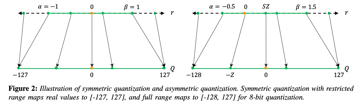
  • asymmetric quantization

    • clipping range에 min/max 값을 사용
      (예로, $\alpha = r_{min}, \beta = r_{max}$)
    • clipping range가 대칭일 필요는 없다.
      ($-\alpha \neq \beta$)

  • symmetric quantization

    • 대칭인 clipping range를 사용한다.
      ($-\alpha = \beta$ = max(|r{max}|,|r{min}|))

    • quantization function의 zero point를 0으로 하여($Z=0$) 수식이 단순화된다.
      $\\$
      $Q(r) = Int(\frac{r}{S})$

  • 

  • asymmetric quantization가 종종 더 tight한 clipping range를 만든다.
    target weights 또는 activations가 imbalanced한 경우 중요하게 고려해야 한다.
    (예를들어, ReLU 이후 activation이 항상 non-negative values를 갖는 경우)

• symmetric quantization에서 scaling factor를 정하는 방식에는 두 가지가 존재한다.

  • "full range" symmetric quantization $S$

    • $S = \frac{2max(|r|)}{2^n-1}$
    • full INT8 range [-128, 127]를 사용
    • 더 정확하며,
      zero point를 0으로 하여($Z=0$) inference중 computational cost가 적기 때문에
      weights를 quantize하는 실전에서 널리 채택됨.
    • 구현이 더 직관적임.

  • "restricted range" $S$

    • $S = \frac{max(|r|)}{2^{n-1}-1}$
    • [-127, 127] range를 사용

• symmetric과 asymmetric quantiation에서 모두 min/max를 사용하는 것이 대세다.
  하지만, 이 접근은 actiation에서의 outlier data에 영향 받을 수 있어서, range를 불필요하게 늘리게 될 수 있다.

  • 이를 해결하기 위한 접근으로 min/max 대신 percentile을 사용하는 연구가 제시됐다.

    • largest/smallest value 대신, i-th largest/smalles values를 $\beta/\alpha$로 사용한다.

  • 또 다른 접근은 real values와 quantized values 사이에서 KL divergence(i.e., infromation loss)를 최소화하는 $\alpha$와 $\beta$를 선택하는 연구[NVIDIA 8-bit inference with tensorRT]가 제시됐다.

  • 참조) 다양한 모델로 calibration methods를 평가한 논문
    Integer Quantization for Deep Learning Inference: Principles and Empirical Evaluation

D: Static vs Dynamic Quantization

"언제 clipping range를 결정할 것인지"

• weight의 clpping range는 static하게 연산되고,
  대부분의 경우에 inference 중에는 parameters는 fixed된다.

• 하지만, activation maps는 각 input sample(아래 수식의 $x$)에 대해서 다르다.
  $\mathcal{L}(\theta) = \frac{1}{N}\sum^N_{i=1}l(x_i, y_i, \theta)$
  그래서 activation을 quantize하는 두 가지 접근이 있다.

  • dynamic quantization

    • clipping range가 각 actication map에 대해 runtime에 dynamically calculated된다.
    • 장점: 각 input마다 정확하게 range를 계산하므로 accruacy가 높다.
    • 단점: real-time computation(min, max, percentile, etc)가 요구되므로 overhead가 크다.

  • satic quantization

    • clipping range가 pre-calculated되고, inference 중에 static하다.

    • 장점: computational overhead가 없다.

    • 단점: dynamic quantization에 비해 accuracy가 낮다.

    • best range를 찾기 위한 다양한 metrics들이 제안되었다.

      • original unquantized weight distriution과, 대응되는 quantized values 간의 MSE(Mean Squared Error)
        (MSE가 가장 popular metric)

      • entropy

      • 신경망 training하면서 clipping range와 weights를 최적화
        LQNets - cited 700+,
        PACT - cited 800+,
        LSQ - cited 500+,
        LSQ+ - cited 150+

E. Quantization Granularity

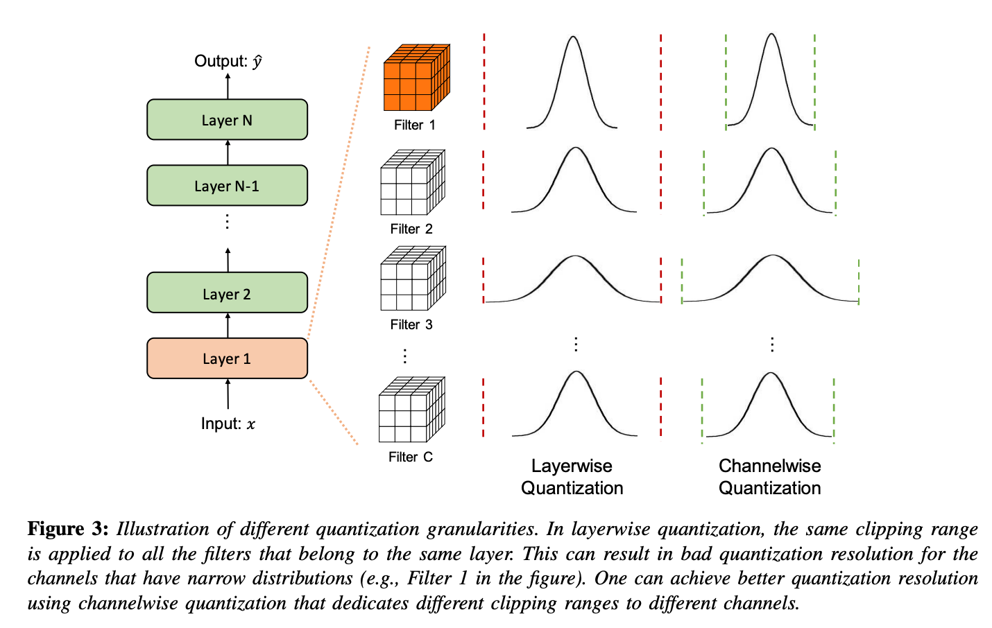
• 위 Figure처럼, 대부분의 컴퓨터 비전 task에서, layer의 activation input은 여러 다른 convolution filter를 거친다.
  각 convolution filter들은 각기 다른 range를 가진 value들을 갖는다.
  이와 같이, weights의 clipping range $[\alpha, \beta]$를 어떻게 세분화해서 계산할 것인지도 quantizaion methods들의 차별화 요소 중 하나이다.

• Category

  • Layerwise Quantization

    • clipping range를 정할 때, layer의 모든 convolution filter들의 weights를 고려한다. (Figure 3)

    • 해당 layer의 모든 parameter의 statistics(min, max, percentile..)을 고려하고,
      모든 convolution filter들에 동일한 clipping range를 사용한다.

    • 구현이 간단하지만,
      각 convolution filter의 range가 다양할 수 있기에, 최적의 accuracy를 갖진 않는다.
      예를 들어, 상대적으로 좁은 parameter range를 가진 convolution kernel은
      동일한 layer에 있는 넓은 range를 가진 kernel로 인해,
      자신의 quantization resolution을 잃을 수 있다.
      

  • Groupwise Quantization

    • layer 안의 다른 여러 channel들을 그룹지어, activation 또는 convolution kernel의 clipping range를 계산한다.

    • 장점: convolution/activation의 parameter들의 분포(distribution)이 넓은 경우(varies a lot)에 유리하다.

    • 단점: 각기 다른 sacling factor들을 계산하는데 추가적인 cost가 필요하다.

    • Q-BERT

  • Channelwise Quantization

    • 다른 channel과 독립적으로, 각 convolution filter에 clipping range로 fixed value를 사용하는 방법이다.
      (Figure 3)

    • 각 channel은 dedicated scaling factor을 할당받는다.

    • 장점: 가장 대중적인 방법이며, (standard method used for quantizing quantizing convolutional kernels.)
      더 나은 quantization resolution과 higher accuracy를 갖는다.

  • Sub-channelwise Quantization

    • Channelwise Quantization은 clipping range가 convolution 또는 fully-connected layer의 any groups of parameters에 대해 결정된다는 점에서 극단적으로(extreme) 사용될 가능성이 있다.

    • 그렇게 되면, single convolution 또는 fully-connected layer를 처리할 때에
      각기 다른 sacling factor들을 계해야 하기 때문에, 상당한 overhead를 일으킨다.

    • 따라서, groupwise quantization은 quantization resolution과 computation overhead 간의 좋은 절충점이 될 수 있다.

• 위 디자인들 간의 trades-off를 설명하는 연구
  Confounding tradeoffs for neural network quantization

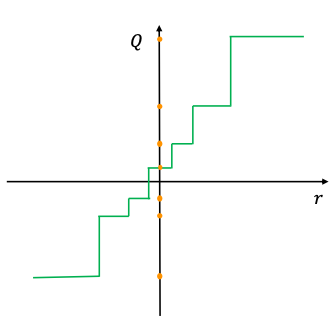
F. Non-Uniform Quantization

• quantization steps와 quantization levers가 non-uniformly sapced되는 quantization이다.
  원래 정보를 더 잘 capture하는 장점이 있지만,
  GPU와 CPU 같은 general한 computation hardware에 효율적으로 적용하기엔 어려움이 있다.
  (그렇기에 uniform quantization이 simple하고 hardware에 mapping하기 효율적이기 때문에, 현재 de-facto이다.)
  

• non-uniform quantizaion의 수식적인 정의는 다음과 같다.
  real number value $r$가 "quantization step $\Delta_i$와 $\Delta_{i+1}$ 사이에 존재할 때, "
  quantizer $Q$가 $r$을 quantization level $X_i$로 projection한다.
  $\\$
  $Q(r) = X_i,$ if $r \in [\Delta_i, \Delta_{i+1})$
  $\\$
  where,
  $Q$: quantizer
  $X_i$: discrete quantization levels
  $\Delta_i$: quantization steps (thresholds)
  $r$: value of real number
  여기서 $X_i$와 $\Delta_i$는 non-uniformly spaced.

• fixed bit-width에서 더 높은 accuracy를 가짐.
  중요한 value 영역에 집중하거나 적합한 dynamic range를 찾음으로써, distributions를 더 잘 파악할 수 있기 때문이다.

• branch(category)

  • brach 1: non-uniform quantization
    weights와 activations의 bell-shaped distribution(종종 long tails를 포함하는)를 사용한다.

  • branch 2: rule-based non-uniform qunaitzation
    quantization steps와 levels가 선형적인(linearly) 증가하는 대신 exponentailly 증가하는
    lograithmic distribution을 사용한다.

  • branch 3: binary code-based quantization
    real number vector $r \in \mathbb{R}^n$이 $m$ binary vectors로 quantized 된다.
    $\\$
    $r \approx \sum^m_{i=1}\alpha_i\bold{b}_i$
    $\\$
    $\alpha_i \in \mathbb{R}$: scaling factor
    $\bold{b}_i \in \{-1, +1\}^n$: binary vectors
    $\\$
    $r$과 $\sum^m_{i=1}\alpha_i\bold{b}_i$ 사이의 error를 최소화하는 closed-form solution은 없기에, 이전의 연구들은 heuristic solution에 의존한다.

  • branch 4: optimization-based non-uniform quantization

    • 최근 연구는 quantizer를 향상시키기 위해,
      non-uniform quantization을 optimization problem으로 공식화 한다.
      아래 수식처럼, original tensor와 quantized counterpart간의 차이를 최소화하도록
      quantizer $Q$ 안의 qunatization steps/levels가 조정된다.
      $\\$
      $min_Q||Q(r) - r||^2$
      $\\$
      Network sketching: Exploiting binary structure in deep cnns
      How to train a compact binary neural network with high accuracy?
      Alternating multi-bit quantization for recurrent neural networks

    • learnable quantizers
      quantizer 자체가 model parameters와 함께 trained된다.
      quantization steps/level가 iterative optimization 또는 graident descent를 통해 trained되는 것이다.
      - iterative optimization
      Alternating multi-bit quantization for recurrent neural networks
      Hessian-aware pruning and optimal neural implant
      - gradient descent
      Learning to quantize deep networks by optimizing quantization intervals with task loss - cited 300+
      Towards accurate binary convolutional neural network - cited 700+
      Quantization networks - cited 300+

  • branch 5: clustering

    • rule-based와 optimization-based의 non-uniform quantization외에도,
      clustering이 quantization으로 인한 information loss를 줄이는데 효과적이다.

    • 각기 다른 tensor에 k-means를 사용해서 quantization steps/levels를 결정하는 연구 방향이 있다.
      Compressing deep convolutional networks using vector quantization - cited 1300+
      [Quantized convolutional neural networks for mobile devices](Quantized Convolutional Neural Networks for Mobile Devices) - cited 1300+

    • Hessian-weighted k-measn cluster을 weights에 적용해 performance loss를 최소화하는 연구도 존재한다.
      Towards the limit of network quantization - cited 200+

G. Fine-tuning Methods

• 신경망을 quantizaion한 이후, parameter들을 종종 조정하는 것(adjust)이 필요하다.
  조정을 위한 방법은 다음과 같다.
  1) 모델을 re-training하는 방법 (= Quantization Aware Training)
  2) re-training없이 조정하는 방법 (= Post-Training Qauntization)
  두 방법의 설계적인 차이는 다음 figure와 같다.
  

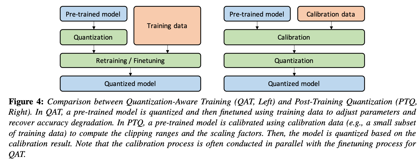
  두 방법의 차이에 관한 연구는 다음을 참고하자.
  A white paper on neural network quantization

• 1) Quantization-Aware Training(QAT)

  • trained model이 주어질 때,
    quantization은 trained model의 parameters에 perturbation을 줄 수 있고,
    이는 model이 floating point precision으로 train될 때 수렴했던 point로부터 멀어지게 만들 수 있다.
    $\\$
    model이 더 나은 loss로 point에 수렴할 수 있도록,
    신경망 model을 quantized parameters로 re-training하는 방법으로 위의 문제를 해결할 수 있다.
    (신경망을 re-training하는데 computational cost가 더 소요된다는 단점이 있다.
    re-training time과 computational cost를 고려했지만, efficiency와 accuracy가 여전히 중요하다면 QAT가 필요할 것이다.)

  • QAT가 가장 popular한 접근으로,
    quantized model에서 forward와 backward pass를 floating point로 수행되지만,
    model parameters는 각 gradient update 이후에 quantized되는 방식이다.
    $\\$
    특히, weight update가 floating point precision으로 수행된 뒤, projection을 하는 것이 중요하다.
    backward pass를 floating point로 수행하는 것이 중요한 이유는,
    quantized precision으로 gradients를 accumulating하면, zero-gradient 문제를 초래하거나, high error를 가진 gradients를 초래한다. (특히 Low-precision에서)

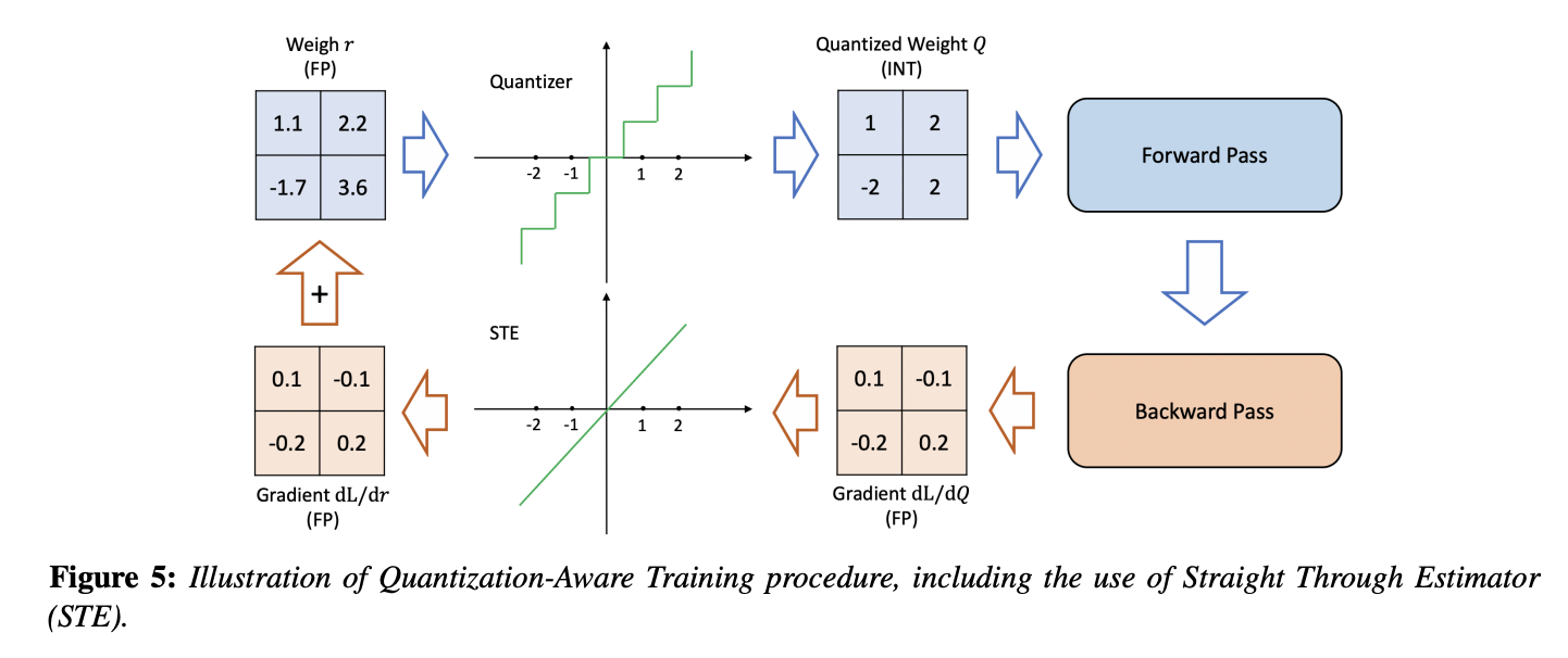
  • STE
    back-propagation에서 중요한 문제는, non-differentiable quantization operator(아래 수식)이 어떻게 다뤄지는지에 대한 문제다.
    
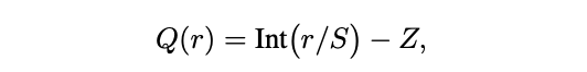
    위 수식의 rounding operation은 piece-wise flat operator이기 때문에,
    어떠한 approximation 없이는, 이 operator의 gradients는 대부분의 곳에서 zero이다.
    $\\$
    이 문제를 다루기 위한 popular한 접근은, Straight Through Estimator(STE)를 이용해서
    operator의 gradient를 approximate하는 방법이다.
    STE는 아래 Figure처럼, rounding operation을 무시하고, identity function으로 approximate한다.
    (identity function: 항등함수, $f(x) = x$)
    

  • STE의 coarse한(거친) approximation에도 불구하고,
    binary quantization과 같은 ultra low-precision quantizaion을 제외하곤, 실전에서 잘 동작한다.
    (참고: 이 현상을 이론적으로 증명한 연구)

  • STE를 사용하는 것이 주요 흐름이지만, 다른 접근들도 연구되었다.
    stochastic neuron으로 STE를 대체한 연구,
    combinatorial optimization을 이용한 연구,
    target propatation을 이용한 안구,
    Gumbel-softmax를 이용한 연구 등이 있다.
    $\\$
    Non-STE methods
    이외에도, regularization opertors를 사용해 weight가 quantized되도록 하는 방법으로,
    아래 quantization 수식에서 non-differentiabl quantization operator를 사용하지 않아도 되는 Non-STE methods 연구도 제안되었다.
    $\\$
    최근 연구 1) ProxQuant
    아래 quantization 수식에서 rounding operation을 제거하고,
    대신 W-shape로 불리는 non0smooth ragularization function을 사용해 weights를 quantization한다.
    
    최근 연구 2)
    pulse training으로 discontinous points의 derivative를 approximate하거나,
    quantized weights를 affine combination of floating point and quantized parameters로 대체한다.
    $\\$
    최근 연구 3) AdaRound
    adaptive rounding method로 round-to-nearest mehtod를 대체한다.
    $\\$
    사실 이런 흥미로운 연구에도 불구하고, STE를 사용하는 접근에 비해 tuning이 많이 필요하기 때문에,
    STE를 사용하는 경우가 보편적이다.

  • model parameters를 조정하는(adjusting)것 외에, QAT 도중에 quantization parameter를 학습하는 것이 효율적임을 발견한 연구들이 있다.
    PACT는 activations의 clipping range를 uniform quantization으로 학습하고,
    QIT는 quantization steps/level를 non-uniform quantization setting의 연장선으로 학습한다.
    LSQ는 새로운 gradient estimate를 도입해서, non-negative activations(e.g. ReLU)d의 sacling factor를 추정한다.
    LSQ+는 general한 activation functions에 위 아이디어를 확장한다.

• 2) Post-Training Quantization (PTQ)

  • 신경망 model을 re-training하지 않고, weights와 activiations quantization parameters가 결정된다.
    

  • QAT에 비해 갖는 장점
    1) expensive한 QAT method를 대체할 수 있는 방법은 PTQ이다.
    PTQ는 어떠한 fine-tuning 없이, quantization과 weights 조정(adjustments)를 수행한다.
    따라서 overhead가 굉장히 낮고, 무시할만하다.
    2) QAT는 retraining을 위해 충분한 양의 training data가 필요하지만,
    PTQ는 제한적이거나 unlabeled data인 경우에도 적용할 수 있다.

  • QAT에 비해 갖는 단점
    QAT와 비교했을 때 상대적으로 낮은 accuracy를 갖는다.
    특히, low-precision quantization의 경우 더욱 그렇다.

  • PTQ의 accuracy를 감소시키는 것을 막기위한 다양한 접근들이 제시됐다.

    • quantization에서 weight values의 mean과 variance 안의 inherent bias를 관찰하고,
      bias correction methods를 제안하는 연구
      Post-training 4-bit quantization of convolution networks for rapid-deployment - cited 500+
      Fighting quantization bias with bias

    • 서로 다른 layer와 channel들간의 weight ranges를 eqaulizing해서 quantization errors를 줄이는 연구
      Recovering neural network quantization error through weight factorization
      Data-free quantization through weight equalization and bias correction - cited 400+

    • quantized tensor와 floating point tensor 간의 L2 distance를 optimize하여 PTQ를 진행하는 연구
      Low-bit quantization of neural networks for efficient inference - cited 300+

    • outlier들의 악영향을 피하기 위해, outlier values를 포함하는 channel을 duplicate하고, halve하는
      outlier channel splitting(OCS) methods를 제안한 연구
      Improving neural network quantization without retraining using outlier channel splitting - cited 300+

    • naive round-to-nearest method를 사용한 quantization 대신,
      adaptive rounding method를 제안해 loss를 줄인 연구.
      quantized weights의 변화를 full-precision counterparts로부터 -1~+1 사이 이내로 제한함.
      AdaRound: Up or down? adaptive rounding for post-training quantization - cited 300+

    • quantized weights가 필요한 만큼 변화할 수 있도록 하는 더 general한 method를 제안한 연구
      AdaQuant: Improving post training neural quantization: Layer-wise calibration and integer programming

• 3) Zero-shot Quantization

  • ZSQ(=Data-Free Quantization)은 quantization 전체를 training/validation data에 대한 access 없이 진행한다.

  • ZSQ는 Machine Learning as a Service(MLaaS)에 특히 중요한데,
    customer의 dataset에 access할 필요 없이, customers'workload의 배포를 가속화하는데 사용될 수 있기 때문이다.
    또한, 보안이나 사생활 문제가 있는 training data를 사용해야 할 경우에 특히 중요하게 사용된다.

  • 지금까지 논의했던 것처럼, quantization 이후 accuracy degradation를 최소화하기 위해선,
    training data의 한 부분 전체를 알아야 한다.

    • 첫 번째로, activations의 range를 알아야 한다.
      values를 clippingg하고, scaling factors를 결정하기 위해서다(calibration을 위해서)

    • 두 번째로, accuracy degradation을 위해선 model parameters를 조정하기 위해 fine-tuning이 종종 요구된다.

    • 하지만, original training data를 아는 것이 quantization 과정 중에는 불가능하다.
      왜냐하면 training datset이 너무 크거나, 보안이 필요한 경우가 있기 때문이다.

      여러 연구들이 이 한계를 다루기 위해 제안되었고, zero-shot quantization이라고 부른다.

  • zero-shot quantization(ZSQ) 의 두 가지 다른 level

    • Level 1: No data and no fine tuning (ZSQ + PTQ)
      ➡️ fine tuning을 하지 않기 때문에, 더 빠르고 쉬운 quantization 가능.

      • weight ranges를 equalizing하고 bias errors를 correcting하여 tlsrudakd model이 어떠한 data나 finetuning 없이 quantization이 더 잘 되도록 하는 연구 - cited 400+

      • 하지만, 이 연구는 scale-equivariance propery of linear activation function에 기반하기 때문에,
        non-linear activations를 갖는 신경망에는 최적이 아닐 수 있다.
        예를 들어, BERT with GELU activation 또는 MobileNetV3 with swish activation

        $\\$

    • Level 2: No data but requires finetuning (ZSQ + QAT)
      ➡️ fine tuning이 quantized model의 accuracy degradation 회복을 돕기 때문에, 더 높은 accuracy를 가짐.

• ZSQ 연구의 popular한 branch는 'target pre-trained model이 훈련한 real data'와 유사한
  synthetic data를 생성하는 연구이다.

  • synthetic data는 quantized model의 calibration, fine-tuning에 사용된다.

  • synthetic data 생성을 위해 GAN을 사용한 연구가 초기에 제시됐다.
    pre-trained model을 discriminator로 사용하여 generator를 훈련한다.

    $\\$

  • generator가 생성한 synthetic data 샘플들을 이용해서,
    quantized model이 fin-tuned 될 수 있도록 full-precision counterpart로부터 knowledge distillation을 이용한다.

  • 하지만, 이 method는 real data의 internal statistics (e.g. intermediate layer activations의 distribution)을 caputre하지는 못한다.
    model의 final outputs만 사용해서 synthetic data를 생성하기 때문이다.
    이러한 internal statistics를 고려하지 못하는 synthetic data는 real data distribution을 적절히 표현하지 못할 것이다.

  • 위 문제를 해결하기 위해, 다양한 후속 연구가 이루어졌다.
    이 연구들은 Batch Normalization(BatchNorm)에 저장된 statistics를 사용한다.
    예로, channel-wise mean과 variance를 사용해 realistic한 synthetic data를 생성한다.
    $\\$
    연구 1) internal statistics의 KL divergence를 direct하게 minimize하고,
    synthetic data를 사용해서 quantized model들을 calibrate하고 finetune한다.
    The knowledge within: Methods for data-free model compression

    연구 2) ZeroQ 연구는 synthetic data를 sensitivity measurement, calibration에 사용하여training/validation data에 access 없이 mixed-precision PTQ를 가능하게 한다.
    ZeroQ 연구는 ZSQ를 object detection task까지 확장시켜서 output labels에 의존하지 않고 data를 생성하기도 한다.
    Zeroq: A novel zero shot quantization framework - cited 300+

    위 두 연구 모두 input images를 trainable parameters로 설정하고,
    이것의 internal statistics가 real data와 유사해질 때까지 directly하게 back-propagation을 수행한다.
    $\\$
    최근 연구) generative models를 train하고 exploit하는 것이
    real data distribution을 잘 capture하고, 더 realistic한 synthetic data를 생성할 수 있음을 발견하고 있다.
    Data-free network quantization with adversarial knowledge distillation
    Generative zero-shot network quantization
    Generative low-bitwidth data free quantization

H. Stochastic Quantization

• inference 중에는, quantization scheme은 주로 deterministic하다.
  하지만, 어떤 연구들은 QAT와 reduced precision training을 위한 stochatsic quantization을 연구하기도 한다.
  Estimating or propagating gradients through stochastic neurons for conditional computation - cited 2600+
  Deep learning with limited numerical precision - cited 2400+

• stochastic quantization이 deterministic quantization보다 신경망이 더 explore 할 수 있도록 해준다는 것이 high-level한 intuition이다.

• rounding operation이 항상 same weights를 return하므로, small weight updates는 어떠한 weight change도 lead하지 못한다는 주장이 위 intuition을 뒷받침한다.
  stochastic rounding을 가능하게 하려면 신경망이 escape할 수 있는 기회를 줄 수 있고, 따라서 parameters를 update할 수 있도록 해야한다.

• stochastic quantization은 weight update 크기와 연관된 probability를 이용해서
  floating number를 up or down으로 mapping한다.
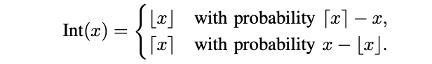
  예를 들어, 아래 두 연구에서는 Int operator(quantization operator)를 아래와 같이 정의한다.
  A statistical framework for low-bitwidth training of deep neural networks
  Deep learning with limited numerical precision. - cited 2400+
  

그런데, 위 정의는 binary quantization에서 사용할 수 없기에, 아래 연구는 수식을 다음과 같이 extend 했다.
BinaryConnect: Training deep neural networks with binary weights during propagations - cited 3400+

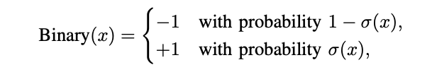
where,
Binary($x$): real value $x$를 binarize하는 함수
$\sigma(\cdot)$: sigmoid function

• 최근에는, QuantNoise 라는 stochastic quantization 연구가 제시됐다.
  각 forward pass에서 각기 다른 random subset of weights를 quantize하고,
  model을 unbiased gradients로 training한다.
  이를 통해 중대한 accuracy drop 없이 lower-bit precision quantization이 진행되도록 한다.
  $\\$

• stochastic quantization methdos의 major challenge는
  모든 각각의 single weight update를 위해 random number를 만들어야 하는 overhead이다.
  따라서 아직 실전에서는 잘 적용되지 않고 있다.

Advance Concepts

: Quantization Below 8 Bits

A. Simulated & Integer-only Quantization

• simulated quantization ( = fake quantization)

  • quantized model parameters는 low-precision으로 저장된다.

  • 하지만, operations(e.g. matrix multiplication, convolutions)는 floating point 연산으로 진행된다.

  • 따라서, floating point operations 이전에
    quantized parameters가 dequantized되는 과정이 필요하다.
    (Figure 6의 중간을 참조하자)

• integer-only quantization ( = fiexed-point quantization)

  • 모든 operations가 low-precision integer 연산으로 수행된다.
    (Figure 6의 오른쪽을 참고하자)

  • 모든 inference가 어떠한 parameters나 activations를 floating point dequantizaion하는 과정 없이
    효율적인 integer 연산으로만 진행된다.

  • 주목할만한 연구로는
    이전의 convolution layer에 Batch Normalization을 fuse하는 연구
    Fixed Point Quantization of Deep Convolutional Networks- cited 990+

    batch normalization과 함께 residual networks에서 integer-only computation하는 연구
    Quantization and training of neural networks for efficient integer-arithmetic-only inference- cited 2800+

    하지만, 두 연구 모두 ReLU activation에 한정되어있다는 점에서 최근 연구로는

    GELU를 approximation하고,
    integer 연산으로 Softmax와 Layer Normalization을 다루며,
    Transformer 구조에 integer-only quantization을 확장 시킨 연구가 존재한다.
    I-BERT: Integer-only BERT Quantization
    
    

  • Dyadic quantization은 integer-only quantization의 다른 class로,
    모든 scaling이 dyadic numbers로 수행된다.
    오직 integer addition, multiplication, bit shifting만 필요하고, integer division은 필요없는 computational graph를 사용한다.
    모든 addition들은 동일한 dyadic sacle를 가지게 하여, logic를 간단하고 효율적으로 만든다는 특징이 있다.

• low-precision logic은 latency, powe consumption, area efficieny 측면에서 이점이 있다.
  아래 Figure 7 왼쪽을 참고해보면, 많은 hardware processor들이 low-precision 연산의 fast processing을 지원하여
  inference throughput과 latency를 boost할 수 있음을 알 수 있다.
  

• 정리하면, integer-only와 dyadic quantization이 simulated quantization보다 더 바람직한 것이 보통이다.
  왜냐하면, integer-only는 lower precision logic을 사용하는 반면에,
  simulated quantization은 floating point logic을 operation에 사용하기 때문이다.
  $\\$
  하지만, compute-bound보다는 bandwidth-bound인 문제인 경우 (예를 들어 추천시스템 같이)
  memory footprint와 parameter를 loading하느 cost가 문제이므로,
  fake quantization을 사용하는 것도 괜찮다

B. Mixed-Precision Quantization

• lower precision quantization을 사용하면 hardware performance가 향상된다.
  하지만, ultra low-precision으로 model을 uniformly quantizing하는 것은 중대한 accuracy degradation을 유발한다.
  이 문제를 Mixed-precision quantization으로 해결한다.

• Mixed-precision quantization에서는
  신경망의 layers들은 quantization에 sensitive/insensitive 한지,
  그리고 각 layer에 사용된 higher/lower bits에 따라 그룹으로 나눈다.
  $\\$
  이를 통해, low precision quantization으로 속도를 높이고 accuracy degradation을 최소화하는 동시에,
  memory footporint를 줄일 수 있다.

• 각 layer는 각기 다른 bit precision으로 quantized된다. (아래 Fig 8처럼)

  • 
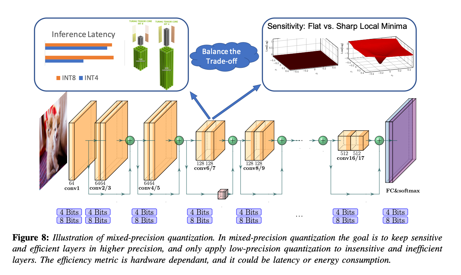
  • Mixed-Precision Quantization의 challenge는 이 bit setting들을 선택할 serach space가 layer의 개수에 지수적이라는 점이다.

• 각 layer에 mixed precision을 선택하는 것은 근본적으로 searching problem이며,
  다양한 연구들이 이를 다루고 있다.

  • 최근, 강화학습을 기반으로 quantization policy를 automatically determine하는 연구가 제시됐다.
    HAQ: Hardware-aware automated quantization - cited 900+

    $\\$

  • mixed-precision configuration search problem을 NAS(Neural Architecture Search)로 formulate하고,
    search sapce를 효율적으로 탐색하기 위해 Differentiable NAS(DNAS)를 사용하는 연구가 제시 되었다.
    Mixed precision quantization of convnets via differentiable neural architecture search

  • 위의 exploration-based 연구들의 단점은 computational resources를 많이 필요로 하고,
    hyperparameter와 심지어 initialization에 성능이 민감한 점이다.

• periodic function regularization을 사용해서 mixed-precision models를 train하는 연구도 있다.
  각기 다른 layers와 layer들의 accuracy와 관한 중요도를 구분하여 train하고,
  layer 각각의 bitwidths를 학습한다.

• 다른 접근의 연구들

  • 1) HAWQ 논문은 model의 second-order sensitivity를 기반으로
    mixed-precision settings를 automatic하게 찾는다.
    second-order operator(i.e. the Hessian)의 trace가 quantization할 layer의 sensitivity를 측정하는데 사용될 수 있음을 밝혔다.

  • 2) HAWQv2는 mixed precision activation quantization으로 확장했다.

  • 3) HAWQv3는 integer-only, hardware-aware quantization으로
    fast Integer Linear programming을 제안해서
    주어진 application specific constraint(model size, latency) 아래 최적의 bit precision을 찾는 연구를 제시했다.
    또한, 이 연구에서 T4 GPUs에 직접적으로 mixed-precision quantization을 적용했을 때의 hard ware efficiency를 다루었고,
    INT4/INT8 mixed precision를 사용해 기존 INT8 quantization보다 50%이상 속도 향상을 이룸을 보였다.

C. Hardware Aware Quantization

• quantization의 목표 중 하나는 inference latency를 향상시키는 것이다.
  하지만, 모든 hardware가 특정 layer/operation이 quantized되었을 때, 동일한 속도 향상을 제공하진 않는다.
  즉, quantization 효과는 on-chip memory, bandwidth, cache hierarchy 등 quantization spped up에 영향을 끼치는 요소들에 hardware-dependant하다.

• 따라서 hardware-aware quantization을 통해 최적의 효과를 달성하는 연구들이 존재한다.
  1) Hardware-aware automated quantization 연구는
  강화학습 agent를 이용해서 quantization을 위한 hardware-aware mixed-precision setting을 결정한다.
  이때 각기 다른 bitwidth를 갖는 다른 layer들에 관한 latency가 담긴 look-up table을 이용한다.
  2) Hawqv3: Dyadic neural network quantization 연구는
  위의 연구가 simulated hardware latency를 사용한다는 점에서,
  직접 hardware 안에서 quantized operations를 실행하고
  실제 각기 다른 quantization bit precision에서 각 layer들의 deployment latency를 측정했다.

D. Distillation-Assisted Quantization

• qunatization의 accuracy를 높이기 위해 Model distillation을 함께 사용하는 연구도 진행됐다.

E. Extreme Quantization

• Extreme low-bit precision quantization은 매우 유망한 연구 방향이다.
  하지만, 현존하는 methods들은 extensive tuning과 hyperparameter search가 수행되지 않는 한,
  baseline과 비교했을 때, high accruacy degradation을 유발하곤 한다.

• Binarization
  Binarization은 quantize values가 1-bit representation으로 한정되기 때문에,
  가장 극적으로 memory requirement를 32$\times$까지 줄일 수 있는
  가장 extreme한 quantization method이다.
  $\\$
  memory 장점 이외에도, binary(1-bit)와 ternary(2-bit) operations는 bit-wise 연산으로 효율적인 연산되고,
  FP32와 INT9같은 higher precision에 비해 더 큰 acceleration이 가능하다.
  $\\$
  따라서 다양한 각기 다른 연구들이 진행됐다.

  • BinaryConnect - cited 3400+
    는 weights를 +1 또는 -1로 제한한다.
    weights는 real values로 유지되고,
    오직 forward와 backward passes 중에만 binarized되어서, binarization effect를 simulate한다.
    $\\$
    forward pass 도중엔, sign function을 바탕으로 real value를 +1 또는 -1로 바꾼다.
    네트워크는 STE를 사용해 non-differentiabl sign function을 통해 gradients를 propagat하여,
    standard training method를 사용해 training한다.

    $\\$

  • BinarizedNN - cited 3300+
    은 weights뿐만 아니라, activations도 binarize한다.
    비싼 floating-point matrix muliplication을 가벼운 XNOR operations과 이후 bit-counting으로 대체해서 latency를 향상시킨다.

  • GXOR-Net은 Binary Weight Network와 XNOR-Net을 제안해서, scaling factor를 weights와 incorporate하고,
    +1/-1 대신 +$\alpha$/-$\alpha$를 사용하여
    (여기서 $\alpha$는 real-valued weights와 binarized weights 간의 거리를 최소화 하기위해 선택된 scaling factor)
    높은 accuracy를 달성한다.
    $\\$
    다르게 표현하면, real-valued weight matrix $W$는 $W \approx \alpha B$로 표현된다.
    ($B$는 아래 optimization problem을 만족하는 binary weight matrix)
    $\\$
    $\alpha, B = argmin||W - \alpha B||^2$
    $\\$

• Ternarization

  • 많은 learnd wights가 zero에 가까운 것을 관측한 것으로부터,
    weights/activations를 ternary values +1, 0, -1로 제한하는 ternariz network 연구가 진행됐다.
    quantized values가 zero가 되도록 명시적으로 허용한 것이다.

  • ternarization 역시 binarization처럼, 비싼 matrix multiplications를 제거해 inference latency를 극적으로 감소시킨다.

  • 이후 Ternary-Binary Network 연구는 binary network weights와 ternary activations의 조합이 accuracy와 computational efficiency 간의 최적의 tradeoff를 달성함을 보였다.

• Reducing the Accuracy Degradation

  • naive binarization과 ternarization methods가 주로 accuracy degradation 문제를 겪고는 한다.
    (특히, 복잡한 task이 ImageNet classification 같은 경우)
    그래서 extreme quantization에서 accuracy degradation을 줄일 수 있는 연구들이 많이 제시되었다.
    Binary neural networks: A survey 연구는 해결책을 세 가지로 분류하였다.

  • 1) Quantization Error Minimization

    • 첫 번째 solution은 quantization error를 최소화하는 방안이다.
      즉, real values와 quantized values 간의 차이를 최소화 하는 연구이다.

    • HORQ과 ABC-Net 연구는 real-value weights/activations를 표현하기 위해 single binary matrix를 사용하는 대신,
      linear combination of multiple binary matrices를 사용하여, quantization error를 줄인다.
      (i.e. $W \approx \alpha_1B_1 + ... + \alpha_MB_M$

    • WRPN,
      One weight bitwidth to rule them all는 activation을 binarizing하는 것이
      연속되는 convolution block의 representational capability를 줄인다는 사실에 착안하여,
      wider networks(filter의 개수가 많은 네트워크)의 binarization이 accuracy와 model size 사이의 good trade-off를 달성함을 보였다.

  • 2) Improved Loss function

    • 두 번째 solution은 loss function을 선택하는데 집중하는 방안이다.
      loss-aware binarization과 ternarization으로 binarized/ternarized weights에 관해 loss를 directly하게 최소화하는 중요한 연구들이 제시됐다.
      오직 weights를 approximate하고 final loss를 고려하지 않은 다른 접근들과 차이를 갖는다.
      Loss-aware weight quantization of deep networks
      Loss-aware binarization of deep networks

    • full-precision teach model로부터 Knowledge distillation을 하는 method 또한
      binarization/ternarization 이후의 accuracy degradation을 회복하는데 도움이 된다.

  • 3) Improved Training Method

    • 세 번째 solution은 binary/ternary models에 더 나은 training methods를 찾는 방안이다.

    • 많은 연구들이 STE가 sign function을 통해 gradients를 backpropagating하는 한계를 지적했다.
      STE는 오직 [-1, 1] 범위 안의 weights/activations를 위해서만 gradients를 propagate 하기 때문이다.

    • 이 문제를 해결하기 위한 연구는 다음과 같다.

      • BNN+
        sign function의 derivative를 continuous approximation하는 방안을 제시했다.
      • Forward and backward information retention for accurate binary neural network(2020),
        Accurate and com- pact convolutional neural networks with trained binarization,
        Blended coarse gradient descent for full quantization of deep neural networks 연구는 sign function을
        sign function을 점진적으로 sharpen하고 approach하는 smooth, differntiable functions로
        대체했다.
        
      • Bi-Real Net은 32-bit activations가 propagated될 수 있는 연속적인 blocks 안에
        activations끼리 연결하는 identity shortcuts를 도입해서,
      • DoReFa-Net은 training 또한 accelerate하기 위해서, weights와 activations 이외에도 gradients를 quantize했다.

• Extreme quantization은 극적으로 inference/training latency를 감소시키고,
  특히 computer vision tasks에서 많은 CNN model size를 줄이는 데 성공적이었다.
  최근에는, 이 시도를 NLP tasks로 확장하여,
  NLP models의 model size와 inference latency를 줄이는 시도가 많이 이뤄지고 있다.
  BERT, RoBERTa, GPT family 등의 large unlabeled dataset에 pre-tranined된 NLP 모델에서
  extreme quantization은 powerful한 tool로 떠오르고 있다.
  

F. Vector Quantization

• quantization 자체는 machine learning에 뿌리를 두지 않는다.
  지난 세기 동안 정보 이론, 특히 digital signal processing field에서 compression tool로 널리 연구되던 분야이다.

• machine learning에서의 quantization이 갖는 주요한 차이점은
  기존의 signal과 최소한의 change/error를 갖는 signal로 compress하는 데에는 별로 관심이 없다.
  대신, reduced-precision representation을 찾아서 loss를 가능한한 작게 만드는 것이 목표이다.
  그렇기 때문에, quantized weights/activations가 non-quantized 값으로부터 멀리 떨어져 있는 것이 크게 상관이 없다.

• 많은 흥미로운 digital signal processing에서의 classical quantizatoin methods의 아이디어들이
  신경망 quantization에 많이 접목되고 있다.
  특히, vector quantization이 그 중 하나이다.
  $\\$
  weights들을 각기 다른 그룹으로 clustering하고,
  inference 과정에서 각 group의 centroid를 quantized values로 사용한다.
  
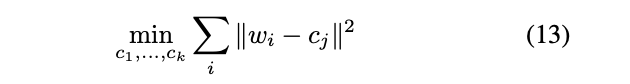
  위 수식에서 $i$는 tensor 안의 weights의 index이고,
  $c_1, ..., c_k$는 clustering으로 찾은 $k$개의 centroid이다.
  또한, $c_j$는 $w_i$에 대응되는 centorid를 의미한다.
  $\\$
  clustering 이후, weight $w_i$는 cluster index $j$를 가진다.
  (loo-up table 안에 있는 $c_j$와 연관된 $j$)

• Compressing deep convolutional networks using vector quantization 연구에서는 k-mean clustering을 사용하는 것이
  큰 accuracy degradation 없이 model sizefmf 8$\times$까지 줄이는데 충분함이 밝혀졌다.
  $\\$
  Deep compression - cited 9500+
  연구에서는 k-means based vector quantizaton을 pruning과 Huffman coding을 함께 사용하면 model size를 더 줄일 수 있음이 밝혀졌다.
  

• Product Quantization
  Product quantization은 vector quantization의 확장이다.
  weight matrix가 submatrics로 나눠지고,
  각 submatrix에 vector quantization을 적용한다.
  $\\$
  basic product quantization 이외에도, clustering을 사용하면 accuracy를 향상 시킬 수 있다.
  Compressing deep convolutional net- works using vector quantization 연구에서는 k-means product quantization 이후 residuals에서 recursive하게 quantized된다.
  Weighted-entropy-based quantization for deep neu- ral networks - 박은혁 교수님, cited 280+
  연구에서는 더 중요한 quantization ranges에 많은 clusters를 적용해서, 정보를 더 잘 보존하는 방식을 사용하기도 했다.

Quantization & Hardware processors

Edge Device's Reosure Constraints

• quantization은 model size뿐만 아니라, faster speed를 가능케 하고,
  특히 low-precision logic을 가진 hardware의 경우 less power를 요구한다.
  그렇기에, quantization은 IoT에서 edge deployment과 mobile applications에 특히 중요하다.

• Edge devices는 compute, memory, power budget과 같은 tight한 resource constraint를 갖는다.
  이러한 제약은 딥러닝 신경망 모델이 맞추기엔 쉽지 않다.
  추가적으로, 많은 edge processor들은 floating point operations를 지원하지 않는다.
  특히, micro-controllers의 경우에는 더욱 그렇다.

Hardware platforms in the context of quantization

• ARM Cortex-M은 low-cost와 power-efficient embedded devices를 위해 고안된
  32-bit RISC ARM processor cores의 group이다.
  $\\$
  예를 들어, STM32 famliy는 ARM Cortex-M cores에 기반한 micro-controller이고,
  edge에서의 신경망 inference에 사용된다.
  $\\$
  몇몇 ARM Cortex-M cores는 floating-point units를 포함하지 않기 때문에,
  딥러닝 model들은 deployment 전에 quantized 되어야 한다.
  $\\$
  CMSIS-NN은 ARM에서 개발한 library로 신경망 모델을 ARM Cortex-M cores상에서 quantize하고 배포하는데 도움을 준다.
  특히, 2의 제곱의 scaling factors로 fixed-point quantization을 leverage해서
  quantization과 dequantization이 bit shifting operation 없이 효율적으로 수행될 수 있도록 한다.
  $\\$
  GAP-8은 dedicated CNN accelerator와 함께 edge inference를 위한 RISC-V SoC(System on Chip)로,
  integer arithmetic만 지원하는 edge processor의 또 다른 예시 중 하나이다.

• 유연성을 가진 programmable general-purpose processor들이 널리 사용되고 있는 반면에,
  purpose-built ASIC chip인 Google Edge TPU는, edge에서 inference를 수행하는 떠오르는 또다른 solution이다.
  엄청난 computing resource를 가진 Google data center Cloud TPUs와는 달리,
  Edge TPU는 small and low-power devices를 위해 디자인 되었기 때문에,
  오직 8-bit arithmetic만 지원한다.
  따라서, 신경망 모델은 TensorFlow의 QAT 또는 PTQ를 사용해서 quantized 되어야 한다.

• 아래 Figure는 edge에서 신경망 inference에 널리 사용되는 각기 다른 commercial edge processor들의 throughput을 나타낸다.

  • 
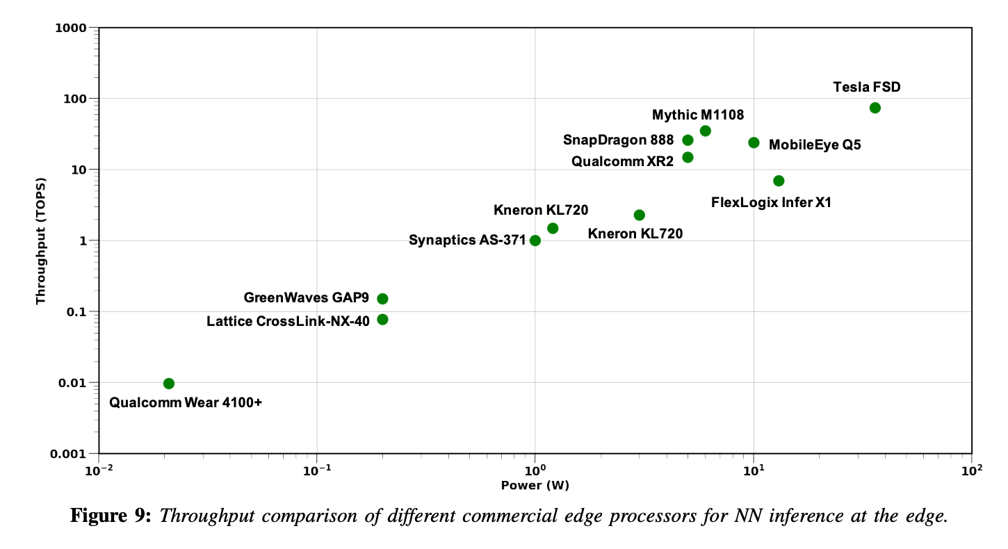
  • 지난 몇년 간, edge processor들의 computing power는 크게 향상됐고,
    costly한 신경망 model의 deployment와 inference를 가능케 만들었다.
    $\\$
    효율적인 low-precision logic와 합한 Quantization과 dedicated 딥러닝 accelerators는
    이러한 edge processor들의 발전을 주도하는 힘이다.

  $\\$

  • quantization in non-edge processors
    quantization은 edge processor에 필수불가결하지만,
    non-edge processor에도 많은 향상을 제공할 수 있다.
    (예를 들어, 99th percentile latency와 같은 SLA(Service Level Agreement) requreimetns)
    NVIDIA Turing GPU는 좋은 예시이며, 특히 T4 GPU는 Turing Tensor Cores를 포함하는데,
    Tensor Cores는 효율적인 low-precision matrix multiplications를 위해 특별히 고안된 실행 unit이다.

FUTURE DIRECTIONS

1) Quantized Software

• 현재 INT8 quantized model(NVIDIA TensorRT, TVM..)은 꽤 optimal하다.
  하지만, lower bit-precision quantization은 아직 많이 available 하지 않다.

• 최근 연구들은 실전에서 low precision과 mixed-precision quantization을 다루고 있다.
  따라서, lower precision quantization을 위한 효율적인 software APIs를 개발하는 것이 하나의 방향이다.

2) Hardware & NN Architecture Co-Design

• classical low-precision quantization과 최근 machine learning에서의 quantization의 주요 차이는
  신경망 parameter가 매우 다른 quantized values를 가져도, 비슷하게 일반화된다는 점이다.
  예를 들어, QAT에서, single precision parameter를 사용해서 original solution과는 동떨어진 different solution으로 converge하더라도, 여전히 good accruacy를 얻을 수 있다.

• 이러한 자유도를 갖는 이점을 활용해서, 신경망 구조를 quantize할 수 있다.
  예를 들어, 최근 연구는 신경망 구조의 width를 변경해서 quantization 이후의 generailization gap을 줄이거나 제거했다.
  One weight bitwidth to rule them all

• 따라서 future work의 방향으로
  depth 또는 individual kernerls와 같은 다른 architecture parameters를 jointly adapt하는 것이 하나의 방향이다.

• 또한, 이를 co-design to hardware architecture로 확장하는 것도 하나의 방향이 되겠다.

3) Coupled Compression Methods

• quantization은 신경망을 효율적으로 배포하기 위한 수단 중 하나일 뿐이다.
  efficient NN architecture design, co-design of hardware and NN architecture, pruning, knowledge distillation과 같은 수단들이 역시 존재한다.

• Quantization은 이러한 다른 수단들과 결합될 수 있다.
  하지만, 현재는 어떤 조합이 최적인지 탐색하는 연구는 매우 적다.
  예를 들어, pruning과 quantization을 모델에 함께 적용해서 overhead를 줄일 수 있다.
  Ps and qs: Quantization-aware pruning for efficient low latency neural network inference(2021)
  Pruning and quantization for deep neural network acceleration: A survey(2021)
  $\\$
  그리고 structured/unstructured pruning과 quantization의 최적의 조합을 이해하는 것이 중요하다.

• 위 방향뿐 아니라, 다른 수단들간의 조합들을 연구하는 것이 future work의 방향이다.

4) Quantized Training

• half-precision으로 신경망을 training하는 것은 매우 중요한 quantization의 역할이었다.
  굉장히 가속화시키고 Power-efficient reduced-precision logic for training을 가능케 했다.

• 하지만, INT8 precision training 아래로 나아가는 것은 굉장히 어려움에 부딪혔다.
  제안된 연구들은 많은 hyperparameter tuning을 요구하거나, 굉장히 소수의 신경망 모델과 쉬운 task에 대해서만 동작했다.

• 본질적인 문제는 INT8 precision에서는 training이 불안정하고, 발산(diverge)하기 때문이다.
  이 challenge를 다루는 것이 edge에서 trainng하는 것에 큰 영향을 미칠 것이다.