[논문 리뷰] Cross-Domain Contrastive Learning for Time Series Clustering

SPS LAB 2025.01.20 논문 세미나

• 본 내용은 Cross-Domain Contrastive Learning for Time Series Clustering 논문을 읽고 정리한 내용입니다.
• 논문 원본은 해당 링크에서 다운받으실 수 있습니다.

Contribution

• temporal domain과 frequency domain information을 통합하는 cross-domain contrastive learning framework 제안
• 클러스터 분포를 정렬하고 시간 도메인의 샘플 범주를 출력하기 위해 도메인 내부 및 도메인 간에 cluster-level constraints을 적용
• 40개의 time series datasets에 대한 실험을 통해 제안된 모델이 우수한 클러스터링 성능을 달성함을 입증

Introduction

• 데이터 구조를 탐색하는 기술인 Data Clustering은 상당한 주목을 받고 있음.
• 특히 image와 text와는 다르게 데이터가 왜곡되거나 이동할 때 유사성 측정을 위해 시계열의 시간적 변화를 충분히 고려해야 하는 게 중요함.
• Dynamic Time Wrapping (DTW), Longest Common Subsequence (LCSS), Pearson correlation coeffcient 등 다양한 방법이 존재하지만, 이러한 방법들은 long-term series clustering을 위한 abnormalities, sensitivity, complexity을 처리하는 데 한계가 있음.
• 또한 기존 딥러닝 기반 시계열 클러스터링 모델은 temporal domain information만 활용하고, 주기적인 패턴을 더 잘 포착하고 노이즈와 이상치에 더 탄력적인 frequency domain information을 활용하지 못하는 문제가 있음.

--> 이를 해결하기 위해 Cross-Domain Contrastive learning model for time series Clustering (CDCC) 방법 제안

Related work

Multi-step Clustering

• Multi-step clustering은 ,K-Means나 hier-archical clustering와 같은 전통적인 clustering 방법 등을 활용하여 time series representation을 추출하는 것을 포함
  • 개선된 LSTM을 사용하여 클러스터링 목적으로 환자 데이터의 장기 의존성을 포착
  • CNN을 활용하여 time series visual images로 변환하여 feature extraction이나 time series clustering을 진행
• 그러나, 이 방법들은 domain-specific하고 universality가 부족하고, feature extraction와 Clustering의 분리는 클러스터링 손실을 통한 특징 추출의 효과적인 안내를 방해

Joint Clustering

• joint clustering은 feature extraction과 clustering을 동시에 최적화하여 호환성(compatibility)을 향상

  • Zhang et al.은 동질적인 클러스터의 시계열이 유사한 subsequence를 공유한다는 가정 하에 다양한 길이의 다변량 shapelet을 사용하여 representation과 class labels을 학습

  • Ma et al.은 feature extraction과 clustering을 반복적으로 최적화하는 self-supervised time series clustering network 제안

  • Ma et al.의 다른 접근으로 특징 추출에서 보간된 값의 분포를 실제 값과 일치시키기 위해 discriminator를 사용하여 clustering error를 최소화하는 것을 목표로 함

• 본 논문에서는 cross-domain contrastive clustering method를 제안. 이 방법은 instance-level 및 cluster-level contrastive constraints에 의해 end-to-end joint clustering을 달성

Contrastive Learning

• self-supervised learning paradigm인 Contrastive learning은 natural language processing, computer vision, recommendation systems 등 다양한 분야에서 사용
• time series 분야에서도 다양한 방향으로 연구가 진행
  • Franceschi et al.에서는 time-based sampling 전략과 유사한 time series는 비슷한 representation을 가질 것이다는 전제의 triple loss를 적용하여 multivariate time series를 처리하는 모델 제안
  • Tonekaboni et al.에서는 인접 지역의 신호가 비이웃 신호와 구별 가능한 distribution을 가져야 한다고 가정하고 debiased contrastive objective에 의해 표현을 학습
  • Eldele et al.에서는 contextual representation을 포착하기 위해 temporal, context를 활용하여 TSTCC라는 time series Contrastive learing framework 제안
  • Yue et al.는 instance와 time scales 간의 시계열을 비교하기 위한 일반적인 프레임워크를 개발
  • 그러나, 언급한 방법들은 frequency domain은 무시하고 temporal domain의 contrastive learning에만 초점을 맞추고 있음
• 본 논문에서는 신호 처리에서 time-frequency transform 기법의 FFT를 활용하여 frequency domain information을 얻고, 이를 통해 temporal domain과 frequency domain 간의 시계열을 cross domain으로 비교하여 중요한 정보를 표현에 통합할 수 있음

Cross-Domain Contrastive Clustering

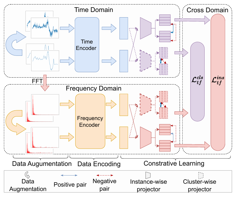
Data Augmentation

• Temporal Domain Data Augmentation
  • time series dataset $\mathbf{X} = \{ x_i \}_{i=1}^{n}$에 대해 random mixing operations을 적용하여 증강 데이터 $\tilde{\mathbf{X}}^t = \{ \tilde{x}_i^t \}_{i=1}^{n}$를 생성
  • $T^a, T^b, T^c$는 jittering, scaling, permutation을 의미하고, $\alpha, \beta, \gamma$는 각각 rate를 의미
  • 본 논문에서는 $\alpha$=0.8, $\beta$=1.1, $\gamma$=0.8로 설정
    $T^a(x_i^t, \alpha), \quad T^b(x_i^t, \beta), \quad T^c(x_i^t, \gamma) \sim \mathcal{T},$

• Frequency Domain Data Augmentation
  • FFT를 활용하여 temporal data를 frequency spectrum으로 변환
    $x_i^f = \text{FFT}(x_i^t).$
  • 이후 frequency components의 추가 및 제거를 포함한 데이터 증강 방법 라이브러리 $F$에 random mixing을 적용
    • frequency components 추가
      • spectrum에서 최대 진폭 $A_m$을 계산
      • $\omega A_m$보다 작은 $\theta$개의 주파수 구성 요소를 무작위로 선택하고 해당 진폭을 $\omega A_m$까지 증가. 여기서 $\omega$는 scaling factor, $\theta$는 perturbation rates를 의미
    • frequency components 제거
      • masking rate $\epsilon$을 사용하여 masking 작업을 사용하여 주파수 구성 요소 무작위로 제거
  • frequency spectrum의 과도한 perturbation은 temporal domain의 큰 변화를 초래할 수 있으며, 각 rate 값들은 너무 큰 값으로 사용하지 않는 것이 중요
  • 본 논문에서는 $\omega = 0.1, \theta = 0.1, \epsilon = 0.1$로 설정
  • $F^a$는 adding, $F^b$는 removing을 나타냄
    $F^a(x_i^f, \omega, \theta), \quad F^b(x_i^f, \epsilon) \sim \mathcal{F},$

Encoding Network

• Encoding Network는 딥러닝에서 time series data의 구조를 포착하는데 중요한 역할을 함

• temporal domain과 frequency domain의 고유한 특성을 활용하기 위해 BiLSTM(bidirectional long short-term memory network)와 three-layer convolutional block를 활용

  • BiLSTM은 time series의 과거와 미래 정보를 모두 고려하고 다양한 기간에 걸쳐 feature를 효과적으로 추출하기 위해 사용

    $H^t = \text{BiLSTM}(X^t), \quad \tilde{H}^t = \text{BiLSTM} (\tilde{X}^t).$

  • Spectrum encoder로 three-layer convolutional block을 활용. Convolutional layer ($Cv1d$), batch normalization layer ($BN1d$), activation function ($relu$), one-dimensional max pooling layer($MaxPool1d$)로 구성

    $CB^3(x_i^f) = CB(CB(\text{Dropout}(CB(x_i^f)))),$
    $CB(x) = \text{MaxPool1d}(\text{relu}(\text{BN1d}(\text{Conv1d}(x)))).$

  • 최종적으로 frequency domain에 대해서 frequency domain representation을 구함

    $H^f = CB^3(X^f), \quad \tilde{H}^f = CB^3(\tilde{X}^f).$

Contrastive Constraints

• Contrastive learing의 최적화 전략은 original sample과 augmented data의 유사도를 최대로, different sample과 유사도를 최소화하는 것

• Instance-level의 contrastive constraint로 InfoNCE loss function으로 설정

  • 인코딩 결과에 직접 적용되지 않고 변환된 표현인 $\{ Z^t, \tilde{Z}^t, Z^f, \tilde{Z}^f \}$에 적용

  • Contrastive loss for sample $z_i^I$의 수식은 아래와 같음. $MLP^2(·)$은 two-layer perceptron, $normalize(·)$는 normalization function, $\tau^I$는 instance-level temperature parameter, $s(z_i, \tilde{z}_i)$는 cosine-similarity

    $\mathcal{L}_{z_i^I} = -\log \frac{\exp(s(z_i^I, \tilde{z}_i^I)/\tau^I)} {\sum\limits_{\substack{j=1, j \neq i}}^n \exp(s(z_i^I, z_j^I)/\tau^I) + \exp(s(z_i^I, \tilde{z}_j^I)/\tau^I)},$
    $z_i^I = g_{\phi}^I(h_i), \quad \tilde{z}_i^I = g_{\phi}^I(\tilde{h}_i),$
    $g_{\phi}^I(h) = \text{normalize}(\text{MLP}^2(h)), \quad h \in \{ h_i, \tilde{h}_i \}.$
    $s(z_i, \tilde{z}_i) = \frac{z_i^T \tilde{z}_i}{\| z_i \| \| \tilde{z}_i \|}.$

  • 최종적인 instance-level contrastive loss

    $\mathcal{L}^{ins}(Z^I, \tilde{Z}^I) = \frac{1}{2n} \sum_{i=1}^{n} \mathcal{L}_{z_i^I} + \mathcal{L}_{\tilde{z}_i^I},$

• Cluster-level의 contrastive constraint로 sample representation에 대해 classification을 진행하여 pseudo-label을 얻음. 이는 유사한 샘플의 집계를 용이하게 하여 모델이 Cluster-level에서 더 차별적인 표현을 학습하는 데 도움이 될 수 있음

  • encoder의 출력에 직접 적용하는 것이 아니라 clustering 결과에 적용

  • $Z_{·,i}^{C}$는 범주 할당 $Z^C$의 i번째 컬럼이라고 하자 ($n$ = 샘플의 수, $k$는 cluster의 수)

  • Cluster-levelcontrastive loss는 아래와 같음. $g_{\phi}^{C}(h_i)$는 two-layer perception과 classification function인 $softmax(·)$를 통해 계산, $\tau^C$는 cluster-level temperature parameter

    $\mathcal{L}_{Z_{i}^{C}} = -\log \frac{\exp(s(Z_{i}^{C}, \tilde{Z}_{i}^{C}) / \tau^C)} {\sum\limits_{\substack{j=1, j \neq i}}^n \exp(s(Z_{i}^{C}, \tilde{Z}_{j}^{C})) + \exp(s(Z_{i}^{C}, Z_{j}^{C}))},$
    $z_i^C = g_{\phi}^{C}(h_i), \quad \tilde{z}_i^C = g_{\phi}^{C}(\tilde{h}_i),$
    $g_{\phi}^{C}(h) = \text{softmax}(\text{MLP}^2(h)), \quad h \in \{ h_i, \tilde{h}_i \}.$

  • degenerate solution을 방지하기 위해 cross-entropy constraints 도입

    $\mathcal{L}_{ce} = - \sum_{i=1}^{k} P_{i}^{C} \log P_{i}^{C} - \tilde{P}_{i}^{C} \log \tilde{P}_{i}^{C},$
    $P_{i}^{C} = \sum_{i=1}^{n} \frac{Z_{i, i}^{C}}{n}, \quad \tilde{P}_{i}^{C} = \sum_{i=1}^{n} \frac{\tilde{Z}_{i, i}^{C}}{n}.$

  • 최종적인 cluster-level contrastive loss

    $\mathcal{L}^{cls}(Z^C, \tilde{Z}^C) = \frac{1}{2n} \sum_{i=1}^{k} \mathcal{L}_{Z_{i}^{C}} + \mathcal{L}_{\tilde{Z}_{i}^{C}} + \mathcal{L}_{ce}.$

Cross-Domain Contrastive Constraints

• temporal domain과 frequency domain 간의 information fusion을 위해 먼저 두 도메인에 instance-level과 cluster-level contrastive constraints를 별도로 적용

• 그런 다음 두 도메인 간의 3번째 contrastive constraints를 설정, 이를 통해 얻은 two-intra-domain loss function은 아래와 같음

  $\mathcal{L}_t = \mathcal{L}^{ins}(Z^I_t, \tilde{Z}^I_t) + \mathcal{L}^{cls}(Z^C_t, \tilde{Z}^C_t),$
  $\mathcal{L}_f = \mathcal{L}^{ins}(Z^I_f, \tilde{Z}^I_f) + \mathcal{L}^{cls}(Z^C_f, \tilde{Z}^C_f).$

• frequency domain representation은 temporal doamin에서 파생되므로 서로 다른 domain에서 동일한 sample의 representation은 유사한 구조적 특성을 가져야 함.

• 이를 위해 도메인 간 증강된 샘플에 대해 instance-level과 cluster-level의 contrastive constraints를 사용. cross-domain contrastive loss function은 아래와 같음

  $\mathcal{L}_{tf} = \mathcal{L}^{ins}(\tilde{Z}^I_t, \tilde{Z}^I_f) + \mathcal{L}^{cls}(\tilde{Z}^C_t, \tilde{Z}^C_f).$

• cross-domain contrastive constraint는 증강된 샘플에만 적용하는데, 원본 데이터에 이를 적용할 시 human labe은 시간 도메인을 사용하여 표시되기 때문에 너무 많은 주파수 도메인 정보를 시간 도메인에 통합하면 클러스터링의 품질이 저하되어 overfitting이 발생하는 문제 발생

• final loss function은 아래와 같음. $\lambda$는 intra-domain constraints와 cross-domain constraint의 중요성을 조정하는 데 사용되는 균형 계수이고, 실험에서는 Adam optimizer와 $\lambda$ 값으로 0.5로 사용

  $\mathcal{L} = \lambda (\mathcal{L}_t + \mathcal{L}_f) + (1 - \lambda) \mathcal{L}_{tf},$

Clustering

• CDCC는 representation learning과 Clustering process를 통합하여 clustering-level representation $Z^c$를 category assignments $Y$의 기반으로 사용하여 다음과 같이 결정.
  $Y = \arg\max \left( g_{\phi}^{C}(\text{BiLSTM}(X)) \right),$
  $g_{\phi}(·)$은 temporal domain에서 clustering-level의 mapping function
• time series data는 temporal information을 기반으로 label이 지정되기 때문에 temporal category output을 최종 결과로 사용. frequency domain data를 레이블링에 사용하는 경우 frequency domain을 사용하는 것을 고려할 수 있음

Experiments

Dataset

제안 방법론의 효과를 입증하기 위해 UCR(University of California, Riverside)의 40 time series datasets으로 실험 진행

Evaluation matrix

Normalized Mutual Information (NMI)와 Rand Index (RI)를 평가 지표로 사용

• NMI (Normalized Mutual Information)
  • 두 확률 분포 간의 상호 정보를 측정하여 클러스터링이 얼마나 정확한지를 나타냄
  • 값의 범위는 0~1이며, 1에 가까울수록 좋은 클러스터링 결과를 의미
• RI (Rand Index)
  • 예측된 클러스터링 결과와 실제 정답을 비교하여 일치하는 정도를 측정
  • 값이 1에 가까울수록 좋은 성능을 의미

Baseline Methods

6개의 semi-supervised, self-supervised model과 4개의 unsupervised representation learning models을 활용

• TSTCC
  • 강력한 augmentation과 약한 augmentation을 도입한 대조 학습 모델로, TST와 유사하게 K-평균 클러스터링을 클러스터링 작업에 적용
• TST
  • Transformer를 기반으로 한 시계열에 대한 unsupervised representation learning 모델로, 회귀, 분류 및 예측에서 supervised method보다 더 나은 성능을 달성
• FeatTS
  • 시계열에서 discriminative feature를 추출한 다음 클러스터링을 수행하는 semi-supervised clustering 방법
• STCN
  • feature extraction 및 clustering을 self-supervised 방식으로 최적화하는 시계열 클러스터링을 위한 self-supervised 네트워크
• R-Clust
  • random convolutions과 PCA(Principal Component Analysis)를 활용하여 특징을 추출하는 시계열 클러스터링을 위한 파이프라인
• TCGAN
  • adversarial game을 사용하여 표현을 최적화하는 시계열에 대한 representation learing 프레임워크

parameter setting

• learning rate, BiLSTM의 레이어 수, 배치 크기, dropout 비율은 논문들의 권장 사항과 실험적 분석을 기반으로 grid search를 통해 최적값을 선택
• temperature parameter $\tau^I = 0.5$, $\tau^C = 1$로 각각 설정

Overall Performance Comparing

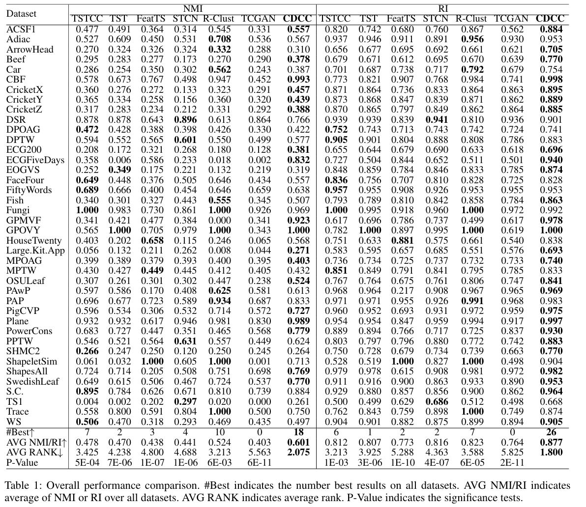
• CDCC 방법은 40개 데이터 세트 중 18개에서 가장 높은 NMI를 달성했으며, 26개에서 가장 높은 RI를 달성
  • 평균 NMI 0.601, 평균 RI 0.877 및 평균 순위 2.075(NMI), 1.800(RI)로 높은 점수를 기록
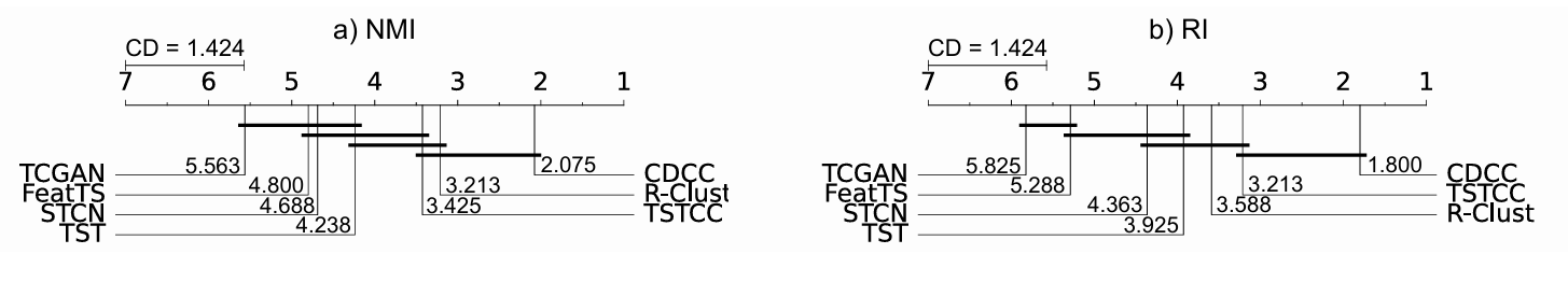
• Bonferroni correction을 사용한 Wilcoxon signed-rank test을 사용하여 CDCC와 다른 방법 간의 쌍별 비교를 수행한 결과, 유의 수준 $p < 0.05$에서 CDCC는 모든 비교 방법에 비해 유의미한 우수성을 보임
• post-hoc Nemenyi tests을 수행한 결과, CDCC는 유의 수준 $p < 0.05$에서 대부분의 baseline에 비해 유의미하게 뛰어난 성능을 나타냄
• TCGA, FeatTS, STCN 및 TST는 NMI 다이어그램에서 수평선을 따라 정렬되어 통계적으로 유의미한 차이 없이 유사한 성능을 보이는 것을 확인
  
• TSTCC는 strong augmentation과 weak augmentation으로 인해 좋은 성능을 보이고, R-Clustering은 많은 수의 random convolutional kernel을 사용하여 특징을 추출하기 때문에 좋은 성능을 보임

Ablation Study

• 모델의 각 구성 요소의 기여도를 분석하기 위해 Ablation Study 진행
  w/o $\mathcal{L}_{tf}^{ins}$: without instance-level cross-domain contrast.
  w/o $\mathcal{L}_{tf}^{cls}$: without cluster-level cross-domain contrast.
  w/o $\mathcal{L}_f$ : without frequency-domain contrast.
  w/o $\mathcal{L}_f \& \mathcal{L}_{tf}$: without both cross-domain contrast and frequency-domain contrast.
  

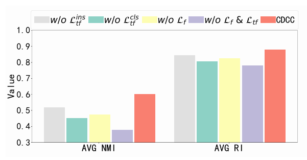
  • instance-level contrast loss나 cluter-level contrast loss를 제거하면 성능이 눈에 띄게 감소
  • frequency-domain loss을 제외하면 cross-domain contrast loss에 대해서만 data representation이 최적화
  • 그럼에도 불구하고 모델의 클러스터링 성능은 cluster-level constraints를 제외했을 때보다 우수
  • cross-domian loss을 추가로 제외하면 모델의 클러스터링 성능이 크게 감소

• 결론적으로 CDCC 모델에서 Cross-domain contrast loss (특히 클러스터 레벨)이 time series의 representation learning에 효과적인 지침을 제공함

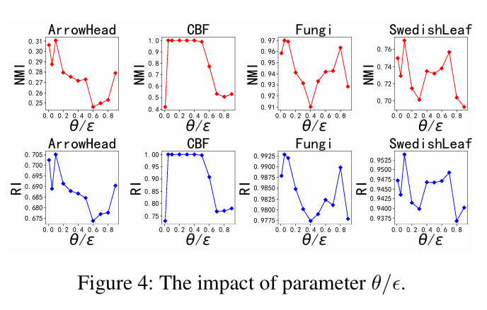
Parameter Analysis

• CDCC의 주요 매개변수인 perturbation rate(θ), masking rate(ϵ) 및 balancing coefficient(λ)를 분석하여 ArrowHead, CBF, Fungi 및 SwedishLeaf 데이터 세트를 사용하여 성능에 미치는 영향을 평가. θ와 ϵ은 모델에서 유사한 역할을 하므로 모든 dataset에 대해 동일하게 설정
• θ와 ϵ의 영향: θ와 ϵ이 증가함에 따라 클러스터링 지표가 지속적으로 변동하는 것을 관찰할 수 있음. 일반적으로 두 값이 작을수록 클러스터링 성능이 향상. 이는 frequency domain information이 augmentation 방법에 민감하기 때문에 frequency components를 과도하게 제거하거나 추가하면 유용한 특징이 손상될 수 있음을 시사
  
• λ의 영향: 데이터셋마다 λ에 대한 민감도가 다름. 일반적으로 λ가 0.5 주변일 때 최적의 클러스터링 결과가 나타나는 경향을 관찰할 수 있음. 이는 cross-domain contrast constraint가 전체 모델 제약 조건에서 중요한 역할을 한다는 것을 시사

Visualization

• Representation Visualization
  • CBF 및 S.C. 데이터셋에 대한 표현 분포를 t-SNE를 사용하여 시각화
    
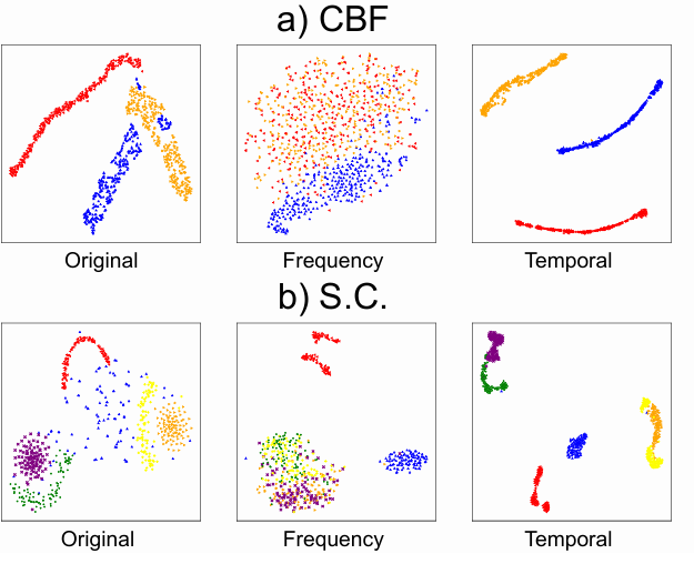
    • original data X는 첫 번째 열에 나와 있는 것처럼 분산되어 있음. T-sne는 사람이 레이블을 지정한 방식으로 데이터 구조를 나타낼 수 없음
    • Frequency domain($H^f$)의 representation도 CBF 데이터셋의 경우 분산되어 있지만, S.C. 데이터셋의 경우 일부 클러스터링 경향을 보임
    • Temporal domain($H^t$)의 representation은 명확한 클러스터링 구조를 보임. CDCC가 사람과 유사한 방식으로 데이터 구조를 발견할 수 있음을 보임.
    • 따라서 주로 temporal domain을 선택하여 clustering categories를 생성
• Convergence Analysis
  • CBF, CricketY, Fungi 및 MOAG 데이터셋을 통해 CDCC의 clustering quality convergence를 보여줌
    
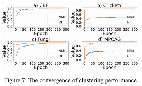
    • Epoch 수가 증가함에 따라 모델의 클러스터링 성능이 꾸준히 향상되어 수렴에 도달하는 것을 확인

Conclusion

• temporal domain과 frequency domain 모두에서 표현 능력을 향상시키기 위해 intra-domain과 cross-domain contrastive constraints을 활용하는 cross-domain contrastive learning model인 CDCC를 제안
• instance-level과 cluster-level의 contrastive constraints을 통합하여 샘플 표현을 최적화하는 것뿐만 아니라 clustering output도 얻음
• 광범위한 실력을 통해 CDCC 모델이 기존 모델보다 전반적으로 우수한 성능을 달성했음을 입증
• Ablation Study에서는 frequency domain information과 cross-domain contrast를 통합하면 클러스터링 성능을 효과적으로 향상시킬 수 있음을 보여줌
• 하지만 이미지나 장치 데이터 등의 비주기적 데이터에 대한 CDCC는 여전히 더 많은 탐구가 필요하며 향후 연구 과제로 존재