pytorch의 기본적인 특징은
Pytorch = Numpy + AutoGrad 이다.
Numpy에만 익숙해도 PyTorch에 반은 익숙한 셈이다.
1. Tensor
Tensor는 PyTorch에서 다차원 Arrays를 표현하는 Pytorch 클래스이다. 사실상 numpy의 ndarray와 동일하다.
numpy- ndarray
import numpy as np
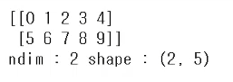
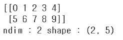
n_array = np.arange(10).reshape(2,5)
print(n_array)
print("ndim : ", n_array.ndim, "shape : ", n_array.shape)output)
pytorch - tensor
import torch
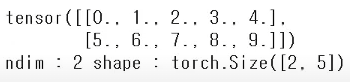
t_array = torch.FloatTensor(n_array)
print(t_array)
print("ndim : ", t_array.ndim, "shape : ", t_array.shape)output)
Tensor 생성은 list나 ndarray를 사용해서도 가능하다.
data(list) to tensor
data = [[3,5],[10,5]]
x_data = torch.tensor(data)
ndarray to tensor
nd_array_ex = np.array(data)
tensor_array = torch.from_numpy(nd_array_ex)
Tensor data types
기본적으로 tensor가 가질수 있는 data 타입은 numpy와 동일하다. 하지만 가장 큰 한가지 차이는 GPU를 사용할 수 있게 해주나 마느냐이다.
Numpy like operations
기본적으로 numpy의 대부분의 사용법이 그대로 적용된다.
data = [[3,5,20],[10,5,50],[1,5,10]]
x_data = torch.tensor(data)

x_data[1:]
#tensor([[10,  5, 50],
#        [ 1,  5, 10]])

x_data[:2,1:]
#tensor([[ 5, 20],
#        [ 5, 50]])

x_data.flatten()
#tensor([ 3,  5, 20, 10,  5, 50,  1,  5, 10])

torch.ones_like(x_data)
#tensor([[1, 1, 1],
#        [1, 1, 1],
#        [1, 1, 1]])

x_data.numpy()
#array([[ 3,  5, 20],
#       [10,  5, 50],
#       [ 1,  5, 10]], dtype=int64)

x_data.shape
#torch.Size([3, 3])

x_data.dtype
#torch.int64
pytorch의 tensor는 GPU에 올려서도 사용이 가능하다.
(나중에 GPU를 이용해서 연산을 돌릴 때 data를 GPU로 옮겨줄 필요가 있다.)
x_data.device
#device(type='cpu')

if torch.cuda.is_available():
	x_data_cuda = x_data.to('cuda')
x_data_cuda.device
#device(type='cuda', index=0)
2. Tensor handling
view, squeeze, unsqueeze 등으로 tensor 조정가능
- view: reshape와 동일하게 tensor의 shape을 변환
- squeeze: 차원의 개수가 1인 차원을 삭제 (압축)
- unsqueeze: 차원의 개수가 1인 차원을 추가
tensor_ex = torch.rand(size=(2,3,2))
tensor_ex
#tensor([[[0.6040, 0.2075],
#         [0.8071, 0.8394],
#         [0.9987, 0.4897]],

#        [[0.9327, 0.6555],
#         [0.7830, 0.5527],
#         [0.6222, 0.0105]]])

tensor_ex.view([-1,6])
#tensor([[0.6040, 0.2075, 0.8071, 0.8394, 0.9987, 0.4897],
#        [0.9327, 0.6555, 0.7830, 0.5527, 0.6222, 0.0105]])

tensor_ex.reshape([-1,6])
#tensor([[0.6040, 0.2075, 0.8071, 0.8394, 0.9987, 0.4897],
#        [0.9327, 0.6555, 0.7830, 0.5527, 0.6222, 0.0105]])
view와 reshape의 출력값이 동일하다. 하지만 view와 reshape는 근본적인 차이가 존재한다.
아래 예제로 확인해보자
view & reshape
a = torch.zeros(3,2)
b = a.view(2,3)
a.fill_(1)
a
#tensor([[1., 1.],
#        [1., 1.],
#        [1., 1.]])

b
#tensor([[1., 1., 1.],
#        [1., 1., 1.]])

a = torch.zeros(3,2)
b = a.t().reshape(6)
a.fill_(1)

a
#tensor([[1., 1.],
#        [1., 1.],
#        [1., 1.]])

b
#tensor([0., 0., 0., 0., 0., 0.])
위의 결과를 보면 view는 얕은 복사(shallow copy)이고 reshape는 깊은 복사(deep copy)임을 알 수 있다.
squeeze, unsqueeze
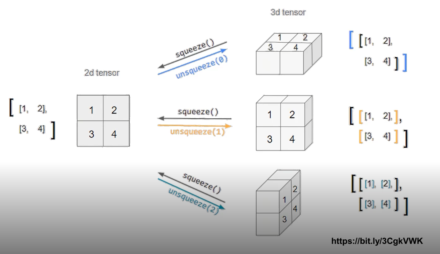
위의 그림과 같이 squeeze는 차원을 줄이고 unsqueeze는 차원을 높이는 역할이다.
unsqueeze에 들어가는 숫자 인자(dim=0,1,2)에 따라 위에서 부터 차례로 (1,2,2), (2,1,2), (2,2,1)로 변하는 것을 확인할 수 있다.
코드 예제도 살펴보자
tensor_ex = torch.rand(size=(2,1,2))
tensor_ex.squeeze()
#tensor([[0.9868, 0.1542],
#        [0.5913, 0.9361]])
tensor_ex.squeeze().shape
#torch.Size([2, 2])
squeeze를 실행해서 2차원의 1 값이 사라진 것을 확인할 수 있다.
tensor_ex = torch.rand(size=(2,2))
tensor_ex.unsqueeze(0).shape
#torch.Size([1, 2, 2])

tensor_ex.unsqueeze(1).shape
#torch.Size([2, 1, 2])

tensor_ex.unsqueeze(2).shape
#torch.Size([2, 2, 1])
3. Tensor operations
기본적인 tensor의 operations는 numpy와 동일하다.
n1 = np.arange(10).reshape(2,5)
t1 = torch.FloatTensor(n1)

t1 + t1
#tensor([[ 0.,  2.,  4.,  6.,  8.],
#        [10., 12., 14., 16., 18.]])

t1 - t1
#tensor([[0., 0., 0., 0., 0.],
#        [0., 0., 0., 0., 0.]])

t1 + 10
#tensor([[10., 11., 12., 13., 14.],
#        [15., 16., 17., 18., 19.]])
스칼라 덧셈은 broadcasting이 일어나 모든 성분에 더해지는 것을 확인할 수 있다.
Tensor operations는 numpy와 마찬가지로 행렬, 백터의 shape가 같아야 가능하다.
행렬곱셈 연산 함수는 dot이 아닌 mm을 사용한다.
n2 = np.arange(10).reshape(5,2)
t2 = torch.FloatTensor(n2)

t1.mm(t2)
#tensor([[ 60.,  70.],
#        [160., 195.]])

t1.dot(t2)
#RuntimeError

t1.matmul(t2)
#tensor([[ 60.,  70.],
#        [160., 195.]])
우선 dot 함수부터 살펴보자
dot 함수는 기본적으로 matrix multiplication을 지원하지 않는다.
반대로 mm 함수는 matrix multiplication만을 지원한다.
또 주목할 점이 matmul과 mm이다.
matmul과 mm은 똑같은 행렬 곱 함수처럼 보이지만 큰 차이를 갖고 있다.
matmul은 broadcasting을 지원하지만 mm은 지원하지 않는다는 점이다.
a = torch.rand(5,2,3)
b = torch.rand(3)
a.mm(b)
#RuntimeError

a = torch.rand(5,2,3)
b = torch.rand(3)
a.matmul(b)
#tensor([[0.2226, 0.4806],
#        [0.1674, 0.2030],
#        [0.1646, 0.4643],
#        [0.4087, 0.5624],
#        [0.4658, 0.3754]])
mm은 연산이 되지 않지만 matmul은 broadcasting을 통해 연산이 된 점을 확인할 수 있다.
4. Tensor operations for ML/DL formula
nn.functional 모듈을 통해 다양한 수식변환을 지원
import torch
import torch.nn.functional as F

tensor = torch.FloatTensor([0.5,0.7,0.1]}
h_tensor = F.softmax(tensor, dim=0)
h_tensor
#tensor([0.3458, 0.4224, 0.2318])

y = torch.randint(5, (10,5))
y_label = y.argmax(dim=1)

F.one_hot(y_label, num_classes=5)
#tensor([[0, 0, 1, 0, 0],
#        [1, 0, 0, 0, 0],
#        [0, 0, 1, 0, 0],
#        [0, 1, 0, 0, 0],
#        [1, 0, 0, 0, 0],
#        [1, 0, 0, 0, 0],
#        [0, 0, 0, 1, 0],
#        [0, 1, 0, 0, 0],
#        [0, 0, 1, 0, 0],
#        [1, 0, 0, 0, 0]])
one_hot 함수에서 num_classes인자는 y_label의 class 개수를 의미한다.
default는 -1로 되어있어서 만약 5번 class에 해당하는 argmax가 없었다면 tensor의 출력값이 5차원의 백터가아닌 4차원의 백터로 표현됐을 것이다.
functional 모듈은 종류가 엄청 방대하기때문에 다 알 필요는 전혀 없다. 기본적으로 필요할 때마다 찾아쓰면 된다.
5. AutoGrad
Pytorch의 핵심은 자동 미분을 지원한다는 점이다.(backward 함수)
w = torch.tensor(2.0, requires_grad=True)
y = w**2
z = 10*y + 50

z.backward()
w.grad()
#tensor(40.)
다음은 백터의 편미분에 대한 예시이다.
a = torch.tnesor([2.,3.],requires_grad=True)
b = troch.tensor(6.,4.], requires_grad=True)
Q = 3*a**3 - b**2

external_grad = torch.tensor([1.,1.])
Q.backward(gradient=external_grad)
pytorch는 numpy와 매우 유사하므로 numpy에 이미 익숙한 사람들은 쉽게 배울 수 있다.
여기까지 기본적인 Basics이고 추가로 필요한 것은 구글링/Document를 통해 찾아보도록 하자