중요한 것 ⭐️

(내 생각에)
1. Motivation - Inspiration
2. Forward / Reverse Trajectory
3. Model probability
4. Training (Paramterization 방법?)
5. Upper & Under bounds of the reverse process's conditional entropy

Introduction

In this post, I'm going to deal with a prior research of DDPM, named DPM : Deep Unsupervised Learning using Nonequilibrium Thermodynamics.

One of the most critical problems in machine learning is a tradeoff between tractability and flexibility.
Tractable distributions mean some probabilistic distributions that can be fit to data easily. On the other hand, flexible distributions mean models that can be fitted to complex structures in arbitrary data.
If given models have a high flexibility, they can reflect structures in arbitrary data, although their log-likelihood can not be computed easily. Also, if the models have a high tractability, they might be analytically evaluated well, but they are unable to aptly describe that.
This phenomenon is the tradeoff between two conflicting things.

In this paper, they propose an approach that achieves both flexibility and tractability by employing two methods : non-equilibrium statistical physics and sequential Monte Carlo (DIFFUSION PROCESS).

Diffusion probabilistic models

This model contributes to the following pros,
1. flexibility in model structure
2. exact sampling
3. easy multiplication with other distribution
4. cheap evaluation of the model log-likelihood

Also, authors develop the methods using ideas from physcis and annealed importance sampling.

Especially, Annealed Importance Sampling (AIS) enable them to define the diffusion process using a Markov chain which slowly converts one distribution into another.

Algorithm

They try to define a forward diffusion process and a reverse diffusion process that matches each other.

Forward Trajectory

First, they set a forward diffusion process, slowly converting a given complex distribution into a tractable one. They define the $q(x^{0})$ and $\pi(y)$ as a data distribution and a tractable distribution, respectively.

Then, they characterize a relationship between these two distributions by the above three equations.
In these equations, $q(x^{(t)}|x^{(t-1)})$ can be represented as either a gaussian diffusion process or a binomial diffusion process.

Reverse Trajectory

In this section, they describe a reverse trajectory.

The given equations are a tractable distribution and a joint distribution, respectively. For both Gaussian and binomial diffusion, this process has the identical functional form as the forward process.

During training, only the mean and covariance are estimated (Gaussian).

Model Probability

Generating data means that models can reflect given data distribution. Therefore, they maximize the log-likelihood of (marginal) data distribution.

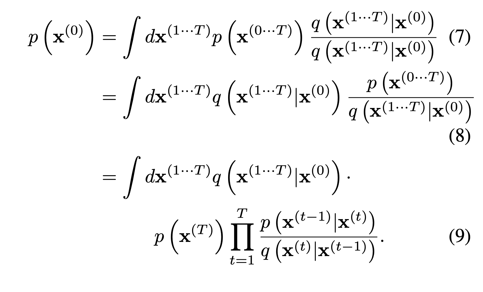
First of all, they attempt to represent data distribution as any form which can match between the forward and reverse process. Thus, they use eq (9).

Training

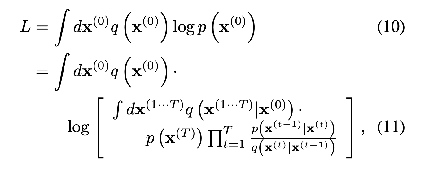
As I mentioned, for train the model, they have to maximize the model log-likelihood.

The log-likelihood can be defined like the above equation, although eq(10) is severely intractable because an integral term is in a log function.
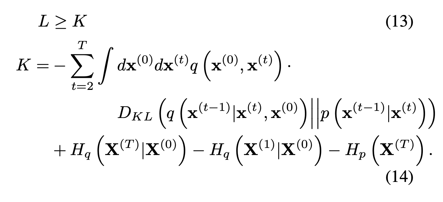
So, they represent the given term eq(12) as lower bound using Jensen's inequality.

In addition, for more straightforward implementation, they finally define the above term.

Resultantly, the objective function is described as the above term.

They parameterize the transition kernel with $\mu_\theta, \Sigma_\theta$

Multiplying Distributions, and Computing Posteriors

Various types of generative tasks like inpainting and denoising require multiplication of the model distribution $p(x^{(0)})$ with a second distribution, or bounded positive function $r(x^{(0)})$.

The core idea in this section is to treat the second distribution as a small perturbation. I'm going to deal with this idea.

Modified Marginal Distributions

The refined probability distribution $\tilde p(x^{(t)})$ can be defined like the above equation. In this equation, $\tilde Z_t$ is a normalization factor.

Modified Diffusion Steps

For sampling, a transition kernel $p(x^{(t)}|x^{(t)})$ should be refined.
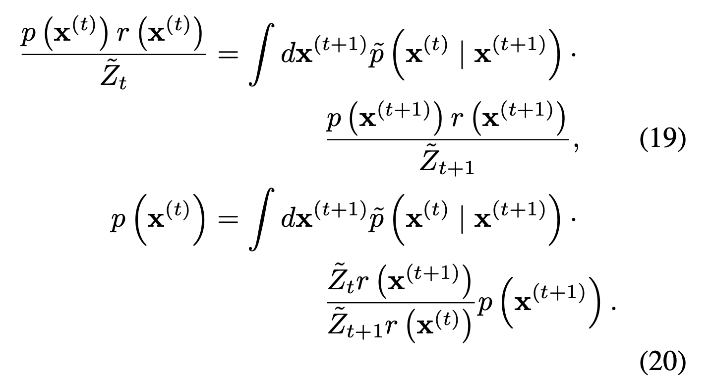
Like the above equation, probabilistic distribution should obey the equilibrium condition.
Thus, refined form also obeys the condition like the above term. Then, applying eq(16) to eq(18), we can derive the below equation.

In this equation(20), for Gaussian, $r(x)$ is smoother than the transition kernel (diffusion step). So, $r(x^{(t+1)})/r(x^{(t)})$ can be seem as a small perturbation to $p(x^{(t)}|x^{(t+1)})$ (ASSUMPTION).

My idea

논문에서는 오피셜로 $r(x)=r(x^{(0)})$으로 정의하여 이 자체를 constant로 생각한다. 즉, inpainting 할 때, 별다른 조치를 취하지 않고 그냥 샘플링 한다는 것이다. 이는 diffusion을 통한 훈련 방법이 이러한 것 자체를 고려할 수 있게끔 한다는 것은 아닐까.
Score function의 관점을 빌려오자면$^{\dag}$, diffusion을 통해 학습된 모델이 절반정도 마스킹된 이미지(부자연스러운 이미지)에 대한 score를 잘 포착한다는 의미..

$^{\dag}$ DDPM과 VE/VPSDE에서 DPM과 denoising score function 사이의 연관성을 보였음.

Entropy of Reverse Process

Authors derive lower and upper bounds on conditional entropy in the reverse trajectory when the forward trajectories are known. The core idea in this section is to treat the second distribution as a small perturbation.

A conditional entropy $H(Y|X)$ means that when a random variable $X$ is given, how much information is needed to describe a random variable $Y$.

The overall development process is in the Appendix of this paper. (The both the upper and lower bound depend only on $q(x^{1...T}|x^{0})$)

If we assume the Gaussian, we can derive the below inequality. https://en.wikipedia.org/wiki/Normal_distribution

This inequality is used in follow-up studies.

생각하면 좋을 부분?

Appendix B.2

위의 eq(14)에서 계산의 편의성을 위해 Lower bound 식을 KL Divergence term과 entropy term으로 바꾼다.

이 과정에서 위와 같은 statement가 나오는데, 여기에서의 edge effects에 대한 설명이 없어서 생각한 바를 적어보려고 함.
Original data $x^{(0)}$을 처음으로 diffusion process에 적용할때 생각해보면 원래 어떤 manifold space 혹은 real space? (맞는 주장인지는 모르겠다.)에 있던 데이터를 $\mu=x^{(0)}$인 Gaussian distribution을 따르게 한다. 하지만 Reverse process의 마지막 스텝인 1->0인 경우 Forward trajectory와 완전히 대응되지 못할 것이라는 걸 알 수 있음..
그래서 여기에서 발생하는 문제가 아닌가 하는 의견.
(이거를 원래 forward trajectory/tractable distribution 가지고 정의하게 되면 결국 훈련에 참여하지 않는 파라미터와 independent한 텀이 되고 사라지게 됨.)