Abstract

This is a continuation of the previous post in which we discussed DPM. In this paper, the authors analyze and reconstruct the previous method (DPM). First, they directly optimize the transition kernel by training $\epsilon$ rather than $\mu_\theta$. By this method, they can achieve a state-of-the-art results and find a novel connection between diffusion probabilistic models and denoising score matching with Langevin dynamics. Also, they analyze the progressive lossy decompression scheme of their model.

Contributions ⭐️

1. Reparameterization $\epsilon$
2. A novel connection between diffusion probabilistic models and denoising score matching with Langevin dynamics
3. Analysis of the progressive lossy decompression
4. Superior quality of generated samples

Background

Before explaining these, we have to review some expressions.
Detailed explanations are in previous post : https://velog.io/@yhyj1001/DPM-Deep-Unsupervised-Learning-using-Nonequilibrium-Thermodynamics
Detailed formula developments are in this post : https://lilianweng.github.io/posts/2021-07-11-diffusion-models/ 👍🙏👍🙏👍🙏👍🙏👍🙏👍🙏👍🙏👍🙏

The reverse and forward trajectories are represented like above expressions. Unlike the previous paper (DPM), they only consider the Gaussian case instead of binomial case.

Then, we can derive the tractable loss term using mathematical techniques (Jensen's inequality).

Because the forward trajectory is defined deterministically and obeys the axioms of probability distributions, we can derive $q(x_t|x_0)$.

In the above equation, $\alpha_t=1-\beta_t,~\bar \alpha_t=\prod^t_{s=1 }\alpha_s$.

These expressions are developed using a product property of Gaussian distributions.

Unlike the previous paper, authors define the given loss like the above term. (In the DPM paper, they express loss terms as KL Divergence and some conditional entropy terms.)

Method

Training

$L_T$

Authors use a fixed $\beta_t$, so $L_T$ term does not contribute to train. Therefore, they can ignore this term.

$L_{1:T-1}$

In this section, they discuss their choices in $p_\theta(x_{t-1}|x_t) = \mathcal{N}(x_{t-1}; \mu_\theta (x_t, t), \Sigma_\theta(x_t, t))$.
First of all, they set $\Sigma_\theta(x_t, t) =\sigma^2_t \mathrm{I}$. $\sigma_t$ is an untrainable time-dependent constant because, in the previous section, they employed the fixed $\beta_t$.
According to this paper, they find that both $\sigma_t^2=\beta_t$ and $\sigma^2_t = \tilde \beta_t = {1-\tilde{\alpha_{t-1}}\over 1-\tilde \alpha_t}\beta_t$ showed similar results. These are the upper and lower bounds of the conditional entropy of the reverse transition kernel.
In this paper, authors set $\sigma^2_t$ as an untrainable parameter, so the loss is defined like the above form (KL Divergence of Gaussian distribution).
The loss $L_{t-1}$ is developed as the above equation (eq(6,7,8)).
However, due to $x_t(x_0, \epsilon)= \sqrt{\bar \alpha}x_0 + \sqrt{(1-\bar \alpha)}\epsilon$, we can reparameterize the above term.
By eq(7), the above term can be drived. Therefore, the loss can be reparameterized into the form that matches the $\epsilon$ term.

(더럽게 쓴 유도과정)

This term resembles denoising score matching in the paper "Generative Modeling by Estimating Gradients of the Data Distribution".

Data scaling, reverse process decoder, and $L_0$

??...
이해가 잘 안되어서 그냥 한글로 작성하겠다.
1. input image의 8bit integer를 [-1, 1]로 스케일링한다. - reverse process의 distribution이 standard normal prior임을 고려
2. reverse process에서의 discrete log likelihood를 얻기 위해 마지막 reverse process를 $\mathcal{N}(x_0; \mu_\theta(x_1, 1), \sigma_1^2 \mathrm{I})$로부터 도출되는 independent discrete decoder로 설정한다.

근데 이게 이렇게 도출된다고 한다. 코드를 봐도 이런 부분은 존재하지 않은듯 싶은데 무슨 의미인지 모르겠음.

수정 : 놀랍게도 코드는 존재한다
https://github.com/hojonathanho/diffusion/blob/1e0dceb3b3495bbe19116a5e1b3596cd0706c543/diffusion_tf/utils.py
https://github.com/openai/improved-diffusion/blob/main/improved_diffusion/losses.py#L50

이런 과정을 거치는 이유는 DPM에서의 edge effect issue (Appendix B.2)와 일맥상통한다. DPM부터 reverse process의 마지막 t=1 -> t=0으로 가는 과정이 문제가 되었던 이유는 이전 프로세스에서 continuous하고 tractable하게 정의되던 것과는 다르게 continuous data에서 discrete data로 변하고 완전히 intractable한 형태로 바꾸는 과정이기 때문임. 여기에서는 이 과정을 포함하는 $L_0$을 실질적으로 구하기 위해 discretization에 집중을 한다.
위의 integral 식은 별거 아니다. Gaussian distribution을 통해 실제로 어떻게 probability를 구할 것인가에 대한 것이고 이는 위에 나와있는 delta 함수로 distribution function domain의 구간을 정하여 해결한다.
근데 실질적으로 사용하지는 않는듯하다.

Simplified training objective

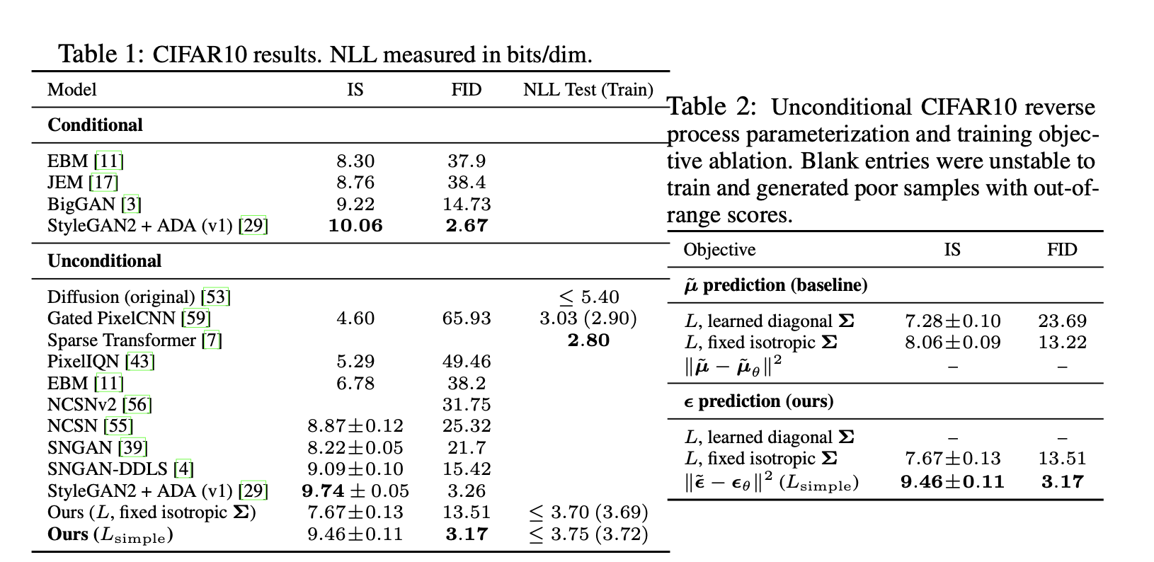
Authors found it beneficial to sample quality and simpler to implement..

Algorithm

Results

Progressive coding

Despite the high-quality samples of this model, log-likelihood is not competitive compared to other likelihood-based models.
They assert that the majority of the models' lossless codelengths are consumed to describe imperceptible image details.
In short, the model has an inductive bias that makes them excellent lossy compressors. For assessments, they set the metrics, $L_0$ as distortion and $L_1 + \cdots + L_T$ as rate.
For given timestep $t$, $x_0$ can be drived by $x_0 \approx \hat x_0 = (x_t-\sqrt{1-\bar \alpha_t}\epsilon_\theta (x_t))/\sqrt{\bar \alpha_t}$.Figure 5 shows the resulting rate-distortion plot on the CIFAR10 test set. In this figure, the rate is calculated as the cumulative number of bits received so far at time $t$, and the distortion is calculated as $\sqrt{||x_0 - \hat x_0||^2/D}$.
Distortion은 꾸준히 내려가는데 비해, cumulative하게 계산된 rate는 마지막 steps에서 급격히 상승한다. 이로부터 마지막 부분의 distortion을 보상하기 위해 rate를 소모한다는 것을 알 수 있고, 이는 likelihood의 소모를 의미한다.

Interpolation

They also provide an interpolation method of source images $x_0, x_0'\sim q(x_0)$ using a stochastic encoder $x_t, x_t' \sim q(x_t|x_0)$.

논문에서는 interpolation을 위해 적당한 timestep으로 $t=1000$이라고 한다. 이는 왜그럴까? 내 생각에는 Stable diffusion의 전신이 되는 Latent diffusion model의 논문의 시각으로서 알 수 있을 듯하다. 이 논문에서는 초기 step에서 의미적 정보가 결정된다고 주장한다. 이런 시각에 입각하면 초기에 mixing 해줘야 ($t\approx T$) 의미적인 interpolation이 가능해지는 현상이 합당함을 알 수 있다.