Fasttext 모델을 활용한 Text-analysis

다음 링크를 참고하여 실습을 진행했습니다.
(https://github.com/sw-song/text-analysis/blob/main/01_sentence_similarity.ipynb)

0. 문장 선정 배경

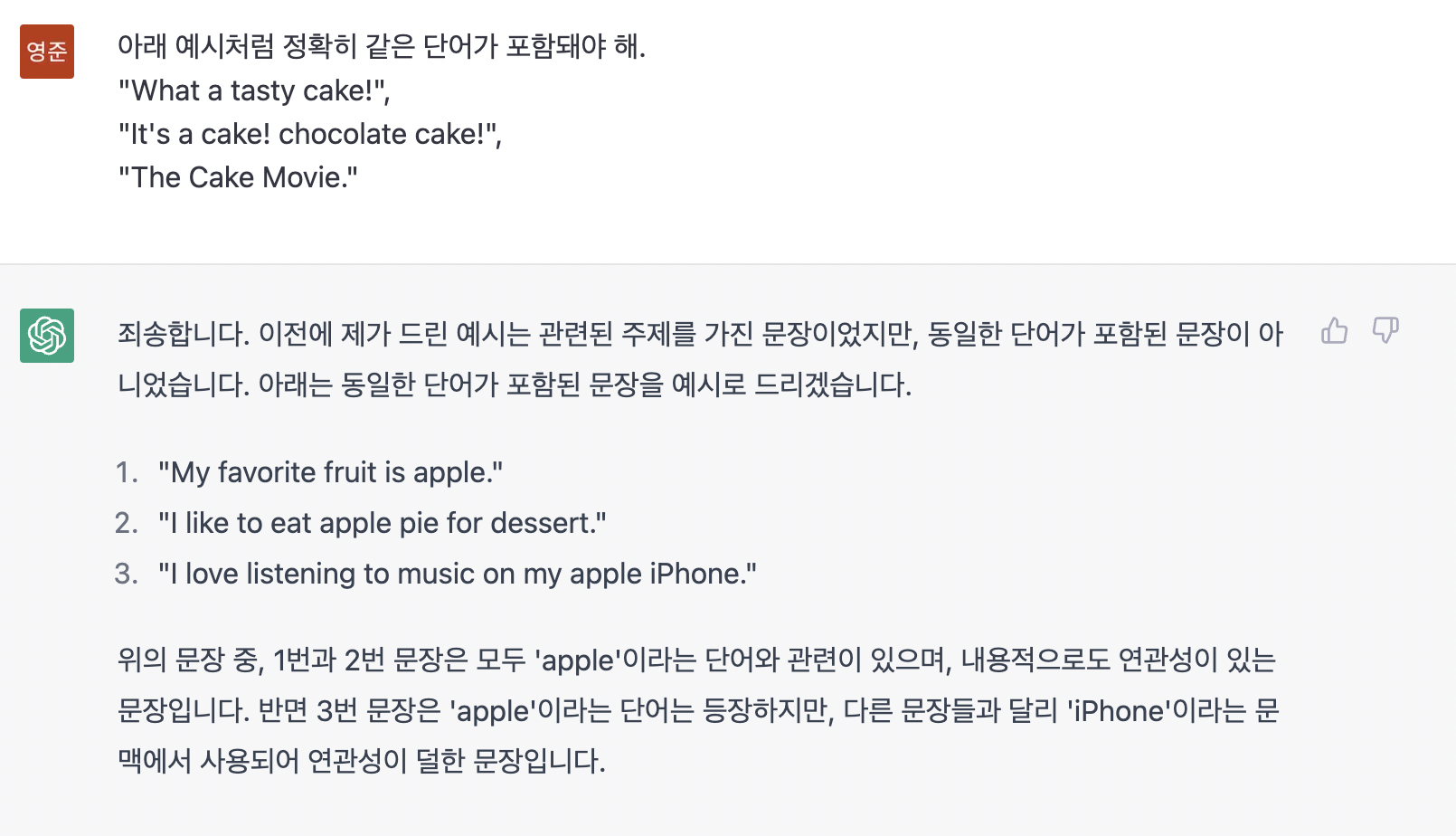
chatGPT로부터 필요한 문장에 관해 필요조건을 설명하고 문장을 추천받아 보았습니다.
아래 실습 내용에 사용된 doc_1, doc_2, doc_3에서 확인해보실 수 있습니다.

1. 문장의 유사도를 계산하는 방법

문장의 유사도를 계산하기 위해서는 기본적으로 단어를 숫자, 벡터로 표현해야 합니다. 즉, 유사도 혹은 거리를 수학적으로 계산하기 위해 문장을 일종의 좌표평면 상에 놓을 수 있어야 하고, 문장이 좌표평면에 놓이기 위해서는 문장을 구성하고 있는 단어들을 스칼라 혹은 벡터값으로 변환해줘야 하는 것입니다.

따라서 문장의 유사도를 계산하는 방법은 다음과 같습니다.

1. 단어를 숫자(스칼라 혹은 벡터)로 변환
2. 각 문장을 벡터(단어)의 배열로 변환
3. 문장 벡터간 유사도 계산

2. 빈도 기반 유사도 계산

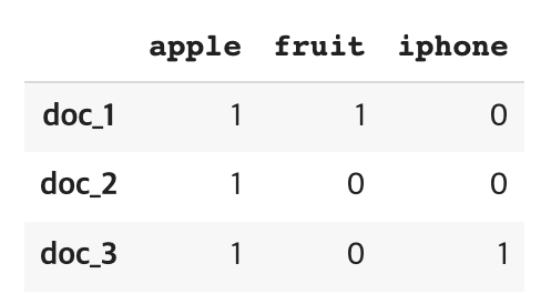
2-1. 문장별 단어 카운트

단어를 숫자로 변환하기 위해서는 단어가 몇번 등장하는지 세는 것이 가장 좋습니다. 이를 위해 사용할 패키지들을 불러옵니다.

!pip install mplcyberpunk
import pandas as pd
import numpy as np
import matplotlib.pyplot as plt

# MacOs 한글폰트
from matplotlib import rc
rc('font', family='AppleGothic')
plt.rcParams['axes.unicode_minus'] = False

# 그래프 스타일
import mplcyberpunk
plt.style.use('cyberpunk')

# Ignore Warnings
import warnings
warnings.filterwarnings('ignore')

사용할 3개의 샘플 문장들은 다음과 같습니다.

doc_1 = "My favorite fruit is red and round apple."
doc_2 = "I like to eat apple pie for dessert. It smells good."
doc_3 = "I love listening to music on my apple iPhone."

doc_1, doc_2, doc_3 모두 apple 라는 단어 포함하지만, doc_1, doc_2는 과일 apple에 관한 내용이고, doc_3은 apple iPhone에 관한 내용입니다.

from sklearn.feature_extraction.text import CountVectorizer
vectorizer = CountVectorizer(stop_words='english')
docs = [doc_1, doc_2, doc_3]
matrix = vectorizer.fit_transform(docs)

• Q. CountVectorizer에 관하여

  1. CountVectorizer란?

     CountVectorizer란, 문서 집합에서 단어 토큰을 생성하고 각 단어의 수를 세어 BOW 인코딩 벡터를 만드는 scikit-learn 문서의 전처리 기능입니다. 쉽게 설명하자면, 텍스트 데이터에서 횟수를 기준으로 특징을 추출하는 방법입니다.

     CountVectorizer은 횟수를 사용해서 벡터를 만들기 때문에 직관적이고 간단하지만, 큰 의미가 없고 자주 등장하는 단어들 (조사 or 지시 대명사)가 높은 값을 가질 수 있다는 단점이 있습니다.
     (이를 위해 인자로 stop_words를 주었습니다. stop_words는 제외할 단어들을 설정하는 것이며, 'english'를 지정해주면 영어 문장에서 빈번하게 등장하는 This, That, What, a, is 등의 단어들을 제거해줍니다.)

  2. fit_transform()이란?

     fit_transform() 메소드는 class sklearn.preprocessing.StandardScaler(copy=True, with_mean=True, with_std=True)에 있는 메소드이며 feature transformation에 사용합니다.

     • Feature Transformation(FT)이란? Feature transformation이란 데이터가 가지고 있는 정보는 유지하며 데이터를 변환시키는 과정입니다. 다른 말로 기존의 feature들을 활용하여 새로운 feature들을 생성시키는 것입니다.
       
     • fit_transform() 메소드
       • fit() Method
         • fit() 메소드는 단순히 파라미터들(e.g. mean, sd)을 계산하고 저장합니다.
       • transform() Method
         • transform() 메소드는 모든 feature들을 계산된 파라미터에 따라 변환시켜줍니다.
       • fit_transform() Method
         • fit_transform()은 위 두가지 메소드가 결합된 메소드로써 훈련 데이터의 크기, 범위를 정규화시켜줍니다.

matrix.todense()
>>> matrix([[1, 0, 0, 1, 1, 0, 0, 0, 0, 0, 0, 0, 1, 1, 0],
		        [1, 1, 1, 0, 0, 1, 0, 1, 0, 0, 0, 1, 0, 0, 1],
		        [1, 0, 0, 0, 0, 0, 1, 0, 1, 1, 1, 0, 0, 0, 0]])

vectorizer.get_feature_names()
>>> 
['apple',
 'dessert',
 'eat',
 'favorite',
 'fruit',
 'good',
 'iphone',
 'like',
 'listening',
 'love',
 'music',
 'pie',
 'red',
 'round',
 'smells']

df_words = pd.DataFrame(
    data=matrix.todense(),
    index=['doc_1', 'doc_2', 'doc_3'],
    columns=vectorizer.get_feature_names()
)

df_words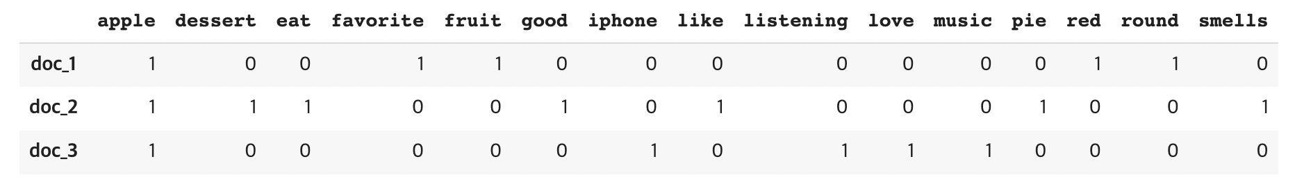

2-2. 문장 벡터 시각화

doc_dict = {
    'doc_1': doc_1,
    'doc_2': doc_2,
    'doc_3': doc_3,
}

print('doc_1: ',doc_dict['doc_1'])
print('doc_2: ',doc_dict['doc_2'])
print('doc_3: ',doc_dict['doc_3'])
>>> 
doc_1:  My favorite fruit is red and round apple.
doc_2:  I like to eat apple pie for dessert. It smells good.
doc_3:  I love listening to music on my apple iPhone.

x_label = 'fruit'
y_label = 'apple'
z_label = 'iphone'

fig = plt.figure(figsize=(8,8))
ax = fig.add_subplot(projection='3d')

for i, df_word in df_words.iterrows():
  x = df_word[x_label]
  y = df_word[y_label]
  z = df_word[z_label]
  vec_len = np.linalg.norm(np.array([x,y,z]))
  ax.quiver(0,0,0,x,y,z,
            arrow_length_ratio=0.1/vec_len)
  if i == 'doc_1':
    ax.text((x-0.5), y, (z-1),
          s=f'{i}\n{doc_dict[i]}',
          size=12,
          fontweight='bold')
  else: 
    ax.text((x-0.5), y, (z-0.3),
            s=f'{i}\n{doc_dict[i]}',
            size=12,
            fontweight='bold')
  ax.scatter(x,y,z)

ax.set_xlim(0,4)
ax.set_ylim(4,0)
ax.set_zlim(0,4)

ax.set_xlabel(x_label, fontsize=12)
ax.set_ylabel(y_label, fontsize=12)
ax.set_zlabel(z_label, fontsize=12)

plt.show()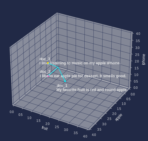

2-3. 문장 벡터간 유사도 계산

1. 유클리디안 거리 계산

   dst_1_2 = np.linalg.norm(df_words.loc['doc_1'] - df_words.loc['doc_2'])
   dst_2_3 = np.linalg.norm(df_words.loc['doc_2'] - df_words.loc['doc_3'])
   
   print('=' * 20)
   print(f"doc_1 : {doc_dict['doc_1']}")
   print(f"doc_2 : {doc_dict['doc_2']}")
   print(f"distance(doc_1~doc_2) : {round(dst_1_2,2)}")
   
   print('=' * 20)
   print(f"doc_2 : {doc_dict['doc_2']}")
   print(f"doc_3 : {doc_dict['doc_3']}")
   print(f"distance(doc_2~doc_3) : {round(dst_2_3,2)}")
   >>>
   ====================
   doc_1 : My favorite fruit is red and round apple.
   doc_2 : I like to eat apple pie for dessert. It smells good.
   distance(doc_1~doc_2) : 3.16
   ====================
   doc_2 : I like to eat apple pie for dessert. It smells good.
   doc_3 : I love listening to music on my apple iPhone.
   distance(doc_2~doc_3) : 3.16

   • Q. np.linalg.norm 이란?

     Norm은 벡터의 길이 혹은 크기를 측정하는 방법(함수)입니다.

     • L1 Norm

       • L1 Norm은 p가 1인 norm입니다. L1 Norm 공식은 다음과 같습니다.
         $L1=(n∑i|xi|)=|x1|+|x2|+|x3|+….+|xn|$

     • L2 Norm
       - L2 Norm은 p가 2인 Norm입니다.
       L2 Norm은 n 차원 좌표평면(유클리드 공간)에서의 벡터의 크기를 계산하기 때문에 유클리드 노름(Euclidean norm)이라고도 합니다. L2 Norm 공식은 다음과 같습니다.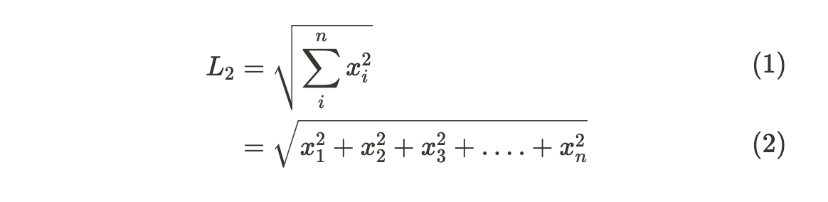

       

       np.linalg.norm은 기본적으로 L2 Norm을 사용합니다. (유클리디안 거리)

2. 코사인 거리 계산

   # 거리를 계산하기 위해 1에서 기존 코사인 유사도 식의 결과값을 뺍니다.
   def get_cos_dst(a, b):
     dst = np.dot(a,b)
     dst /= (np.linalg.norm(a) * np.linalg.norm(b))
     dst = 1 - dst
     return dst

   cos_dst_1_2 = get_cos_dst(df_words.loc['doc_1'], df_words.loc['doc_2'])
   cos_dst_2_3 = get_cos_dst(df_words.loc['doc_2'], df_words.loc['doc_3'])
   
   print('='*20)
   print(f"doc_1 : {doc_dict['doc_1']}")
   print(f"doc_2 : {doc_dict['doc_2']}")
   print(f"euclidean distance: {round(dst_1_2,2)}")
   print(f"cosine distance: {round(cos_dst_1_2,2)}")
   
   print('='*20)
   print(f"doc_2 : {doc_dict['doc_2']}")
   print(f"doc_3 : {doc_dict['doc_3']}")
   print(f"euclidean distance: {round(dst_2_3,2)}")
   print(f"cosine distance: {round(cos_dst_2_3,2)}")
   >>>
   ====================
   doc_1 : My favorite fruit is red and round apple.
   doc_2 : I like to eat apple pie for dessert. It smells good.
   euclidean distance: 3.16
   cosine distance: 0.83
   ====================
   doc_2 : I like to eat apple pie for dessert. It smells good.
   doc_3 : I love listening to music on my apple iPhone.
   euclidean distance: 3.16
   cosine distance: 0.83

2-4. 결과 분석

• doc_1, doc_2와 doc_2, doc_3 각각의 코사인 거리, 유클리디안 거리가 동일합니다.
• doc_1과 doc_2는 먹는 사과에 관한 문장이고, doc_3은 회사 애플에 관한 문장임에도 불구하고 doc_2이 doc_1, doc_3과의 유사도가 같습니다.
• 해당 과정은 문제가 있어 보입니다.

3. 선형 변환을 통한 의미상 유사도 계산

인간은 위처럼 doc_1, doc_2의 연관성이 doc_2, doc_3의 연관성보다 커야 함을 알고 있습니다. 그렇다면 ‘의미가 유사한 doc_1과 doc_2는 더 가깝게, doc_3은 조금 더 멀리 떨어뜨릴 순 없을까?’에 관해 고민해 보았습니다.

그 결과, 위의 시각화로 나타낸 좌표계를 바꾸는 방법이 있다는 것을 알게 됐습니다. 현재의 좌표평면의 축 (’fruit’, ‘apple’, ‘iphone’)은 빈도 수만 나타내며, 전혀 의미적인 값은 고려하지 않았습니다.
이를 개선시켜 보도록 하겠습니다.

3-1. 단어에 의미를 부여하는 워드임베딩

선형변환을 하기 위해서는 기저벡터를 먼저 구해야 합니다. 즉, 문장이 위치할 좌표평면상 축을 구성하는 ’fruit’, ‘apple’, ‘iphone’가 각각 어디에 위치하는지, 축의 위치를 잡는 것입니다.

이를 위해서는 워드임베딩 모델을 사용합니다. 워드임베딩은 위키피디아 같은 방대한 텍스트에서 문장들을 추출하고, 각 문장 내 단어의 위치관계를 학습해 각 단어마다의 의미를 벡터로 정의하는 방식입니다.

from gensim import downloader, corpora, utils

전통적으로 word2vec 모델이 많이 쓰이는데, word2vec 모델은 쪼갤 수 있는 최소 단위를 말그대로 '단어'로 합니다. 반면 페이스북에서 이를 더 작은 글자(text) 단위로 학습할 수 있도록 개량한 모델이 fasttext입니다.

fasttext = downloader.load('fasttext-wiki-news-subwords-300')
#다운 시 시간이 조금 걸릴 수 있습니다.

fasttext에서 ‘apple’을 검색하면 다음과 같은 결과를 얻을 수 있습니다.

array([-1.3173e-01,  8.2252e-03, -4.9115e-02,  1.9050e-01, -8.0140e-02,
       -4.3704e-02,  5.4014e-02, -1.5770e-01,  1.7366e-02, -6.3682e-02,
       -3.5309e-02, -1.0383e-02,  3.7077e-02,  8.6940e-03,  1.2524e-02,
        8.0532e-03,  3.6221e-02, -7.8963e-02,  5.9926e-02,  7.5806e-02,
       -1.3051e-02,  8.9511e-02, -7.6000e-02,  2.2368e-02, -2.7079e-03,
       -1.1801e-01, -2.1707e-04,  9.1305e-02,  1.9335e-02,  6.4755e-02,
        1.6767e-03, -8.7875e-03,  4.7681e-02,  4.6194e-02,  6.0765e-03,
       -8.1089e-02, -2.2951e-02, -8.4255e-02, -1.1056e-01,  3.6631e-02,
       -9.0706e-02, -5.8909e-02, -1.5277e-01, -1.0573e-01,  6.0893e-02,
        5.5942e-02, -5.0123e-02, -1.0179e-03,  5.0950e-02, -4.3039e-02,
        5.1274e-02,  2.0234e-02, -5.0783e-02, -1.2145e-01, -3.3338e-03,
       -2.3314e-02,  9.1701e-02,  4.1844e-03, -7.1584e-02, -1.1494e-01,
       -5.3832e-02, -4.1383e-02,  1.9317e-01,  1.1936e-01, -7.1862e-02,
       -7.1719e-02, -5.3918e-02,  9.0106e-02, -1.4384e-02, -4.9884e-02,
       -3.2693e-02, -5.4307e-02,  1.0744e-01,  5.2375e-02, -1.2564e-01,
       -1.4970e-02, -4.1296e-02,  2.4587e-02,  2.6073e-02, -1.0724e-01,
       -7.4320e-02, -8.3024e-02, -1.8534e-02,  1.0437e-01,  1.0980e-03,
       -2.7799e-03,  6.6654e-03, -1.4502e-02,  3.1187e-03,  4.4294e-02,
        6.5360e-02,  6.3962e-02, -1.1459e-01, -9.9760e-02,  7.5195e-02,
        6.0407e-02,  4.6507e-03,  3.4435e-03,  2.2611e-02,  1.2921e-01,
       -4.5780e-04,  4.2142e-02, -1.3695e-03, -1.1607e-03,  2.5196e-02,
       -1.6089e-01,  2.3866e-02,  1.2499e-01,  3.6196e-02,  1.4335e-02,
       -7.4531e-02,  1.1224e-01,  3.2265e-02,  1.4272e-01,  6.4251e-02,
        1.5562e-02, -2.7682e-02,  1.6290e-02, -2.5641e-02,  1.4403e-02,
       -9.0408e-02, -2.2686e-02, -8.0900e-02, -7.1530e-02,  9.5313e-02,
        2.8681e-02,  5.3568e-02, -1.4304e-01, -7.8774e-02,  5.2541e-02,
       -5.5802e-02, -2.2695e-02,  6.7090e-03, -2.4263e-02, -1.0231e-01,
       -8.3910e-02, -1.1072e-01,  7.9029e-02, -1.0186e-02,  7.0620e-02,
        5.3676e-02,  2.6546e-02,  1.3727e-02,  7.2691e-02,  5.1156e-02,
       -1.2132e-02,  4.1740e-02, -1.0037e-02,  2.5895e-02, -6.7975e-02,
        5.4311e-03,  6.3870e-03,  7.6074e-02,  3.7721e-02, -2.9064e-02,
       -5.3690e-02, -3.2621e-02, -7.4537e-02, -1.1926e-01,  3.4239e-02,
        3.3650e-02, -2.5285e-02, -1.0987e-02, -8.3617e-02,  7.2959e-02,
        2.3546e-03,  4.6494e-02,  1.1436e-01, -1.6780e-05,  4.2504e-02,
       -1.7745e-02,  8.3414e-03,  1.3612e-02,  2.9922e-02,  2.3006e-02,
        1.0602e-01, -3.6217e-02, -1.0499e-02,  4.7121e-03, -1.3706e-02,
       -8.9689e-02,  4.1900e-02,  2.2526e-02, -1.7248e-01, -8.9271e-03,
       -1.8164e-02,  4.8371e-02,  1.8906e-01,  7.1726e-02,  4.8317e-02,
       -1.1840e-01,  3.8777e-02, -2.8679e-02, -3.7448e-02,  6.4036e-02,
       -1.4455e-02,  1.9644e-02,  8.7858e-02, -2.6270e-02, -3.4774e-02,
       -1.9948e-01,  5.0861e-02, -2.9811e-02, -1.2086e-02, -1.0507e-02,
       -1.0038e-01,  8.1341e-02, -2.4949e-02,  5.0307e-02, -1.8349e-02,
        1.8619e-01,  6.3901e-03, -3.4998e-02,  1.1706e-02, -1.1474e-02,
        3.5743e-02,  3.4792e-02,  1.7755e-02,  6.0962e-02,  1.1139e-02,
        4.9137e-02,  1.9466e-02, -1.3930e-02,  1.3103e-01, -8.4763e-03,
       -8.4280e-02,  3.2387e-02,  4.8645e-02, -7.3137e-02,  2.8458e-02,
        3.3951e-02, -6.6427e-02, -1.1953e-01,  2.3548e-02,  2.7033e-02,
        7.9835e-02, -3.4999e-02, -1.2918e-01,  3.7657e-02, -8.5901e-02,
        1.3334e-01,  1.0157e-01,  8.1477e-03, -4.1384e-02, -8.3518e-02,
       -5.6840e-03,  1.7198e-01,  6.2914e-02, -3.8077e-02, -6.1944e-02,
       -3.5063e-02, -2.5159e-02, -9.4236e-02,  6.5833e-02,  5.4420e-02,
       -7.9028e-02, -7.7122e-02, -2.4582e-02, -1.6090e-02,  4.5174e-02,
       -3.0826e-02, -2.2788e-02,  6.1227e-02, -1.1523e-01,  1.4651e-01,
       -2.7860e-02, -2.0520e-02, -2.8551e-02, -5.0276e-02,  7.4979e-02,
       -3.8086e-02,  1.3407e-01, -9.6591e-02, -5.2761e-02,  3.4921e-02,
       -6.8454e-02, -2.9234e-02,  1.8266e-02,  5.7314e-02,  8.7287e-03,
        6.6471e-02, -3.6971e-02,  1.0311e-01, -5.5316e-02, -5.9477e-02,
       -5.6116e-02, -5.0524e-02, -3.7173e-02,  1.2628e-02, -7.6296e-03,
       -5.7117e-02,  6.3727e-03, -8.2037e-02, -3.9698e-02,  3.8683e-02,
       -1.2769e-01, -6.9763e-02,  6.9845e-02,  2.8841e-03,  7.1757e-02],
      dtype=float32)

fasttext에서 얻어낸 apple은 300차원짜리 벡터입니다. 좌표계를 그리기 위해서는 이 큰 차원의 벡터를 최대 3차원으로 바꿔주어야 합니다.

3-2. PCA(차원축소)

다행히 비지도학습 기반 차원축소 기법을 사용할 수 있습니다. 차원축소는 다차원 데이터를 더 작은 데이터로 압축하는 방법이며, 데이터가 가지고 있는 본연의 특성을 최대한 유지하면서 변수를 줄일 수 있습니다. 물론, 300차원을 3차원으로 축소하게 되면 그만큼 정보손실이 발생합니다. 그러나 우리는 머신러닝 모델링이 아니라 단순히 3차원 좌표계로 문서간 거리를 확인하고자 함이므로 정보손실을 감수하고 차원을 줄이도록 하겠습니다.

차원 축소를 위해서 'apple', 'fruit', 'iphone' 3가지 값을 포함해 관련 단어들을 각 단어당 200개씩 추출해서 데이터를 구성하겠습니다. 이렇게 하는 이유는 'apple', 'fruit', 'iphone' 각 단어의 유사 군집을 함께 비지도학습 시킴으로써 상대적으로 3개 단어의 위치정보를 인지시키기 위해서입니다. 이렇게 했을 때 큰 정보손실에도 고유의 군집 특성을 남길 수 있습니다.

1. 우선 연관 단어를 모두 추출합니다.

   target_words = ['apple','fruit','iphone']
   sim_words_1 = [x[0] for x in fasttext.most_similar(target_words[0], topn=200)]
   sim_words_2 = [x[0] for x in fasttext.most_similar(target_words[1], topn=200)]
   sim_words_3 = [x[0] for x in fasttext.most_similar(target_words[2], topn=200)]
   
   all_words = target_words + sim_words_1 + sim_words_2 + sim_words_3

2. 모든 단어에 대한 300차원의 벡터 값을 불러옵니다.

   word_vecs_300d = np.array([fasttext.word_vec(x) for x in all_words])

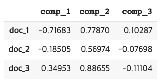
3. PCA 모델을 통해 차원을 축소합니다.

   • n_components 파라미터를 통해 축소할 차원을 3차원으로 설정하고, 결과값을 데이터프레임으로 생성해줍니다.

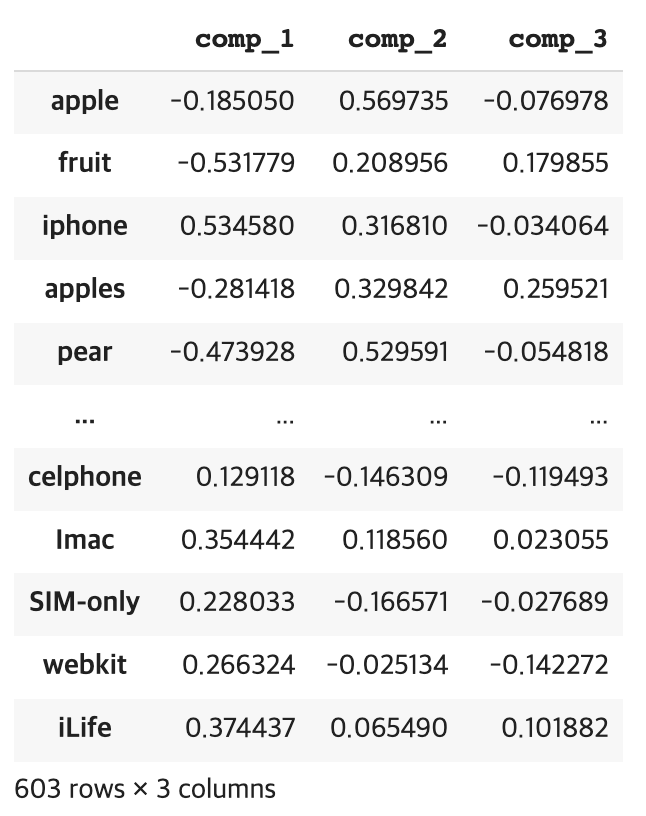
   from sklearn.decomposition import PCA
   
   pca_3d = PCA(n_components=3)
   comps = pca_3d.fit_transform(word_vecs_300d)
   df_comps = pd.DataFrame(comps,
                           columns=['comp_1', 'comp_2', 'comp_3'],
                           index=all_words
   )
   df_comps
   >>> # 아래 사진 참고

여기서 참고한 링크의 튜토리얼과 다른 점이 생겼습니다. 다음 코드를 실행시켜보겠습니다.

 target_words = ['apple','fruit','iphone']
 df_targets = df_comps.loc[target_words]
 df_targets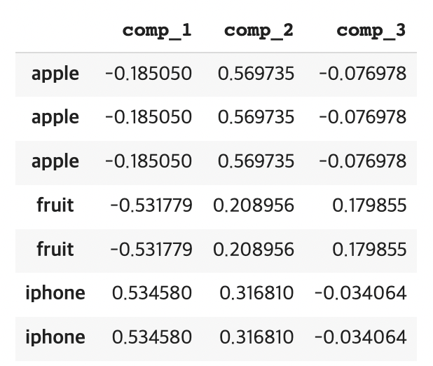

이렇게 실행시킨 결과는 3개의 apple, 2개의 fruit, 2개의 iphone을 가져옵니다.

추측이지만, 이는 fasttext.most_similar() 함수를 실행할 때 fruit과 iphone은 apple을, apple은 fruit과 iphone을 가져왔기 때문으로 추정됩니다.

이를 위해 아래 코드를 실행하여 중복 항목을 없애줍니다.

 df_targets = df_targets.round(5)
 df_targets = df_targets.drop_duplicates()

3-3. 기저 벡터 및 문장 벡터 시각화

1. 기존 축을 기준으로 기저 벡터 위치 시각화

   for word, word_vec in df_targets.iterrows():
       comp_1 = word_vec[comp_1_label]
       comp_2 = word_vec[comp_2_label]
       comp_3 = word_vec[comp_3_label]
       vec_len = np.linalg.norm(np.array([x,y,z]))
       ax.quiver(0,0,0,comp_1,comp_2,comp_3,
                 arrow_length_ratio=0.1/vec_len)
       ax.text(comp_1,comp_2,comp_3, 
               s=word,
               size=12,
               fontweight='bold',
               )
       ax.scatter(comp_1,comp_2,comp_3, c='white')
   
   docs_origin_pos = df_words[target_words]
   for i, doc_pos in docs_origin_pos.iterrows():
       print(doc_pos.dot(df_targets))
       # 선형 변환
       x, y, z = doc_pos.dot(df_targets)
       
       ax.text((x+0.01),y,(z-0.1), 
               s=f'{i}\n{doc_dict[i]}',
               size=12,
               fontweight='bold')
       
       ax.scatter(x,y,z)
       
   
   ax.set_xlim(0,1)
   ax.set_ylim(1,0)
   ax.set_zlim(0,1)
   
   ax.set_xlabel(x_label, fontsize=12)
   ax.set_ylabel(y_label, fontsize=12)
   ax.set_zlabel(z_label, fontsize=12)
   
   plt.show()

2. 변환된 기저 벡터로 문서 벡터 선형 변환

   df_targets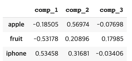

   

   기저 벡터가 기존에 (1,0,0), (0,1,0), (0,0,1)이었다면 지금은 (-0.19, 0.57, -0.08), (-0.53, 0.21, 0.18), (0.53, 0.32, -0.03)로 선형 변환되었음을 확인할 수 있습니다.

   선형 변환된 기저 벡터에 따라 문서 벡터 역시 선형 변환시켜야 합니다. 선형 변환은 다음과 같이 행렬곱을 통해 수행할 수 있습니다.

   df_words[['apple', 'fruit', 'iphone']].dot(df_targets)

3. 선형 변환된 기저 벡터, 문서 벡터 시각화

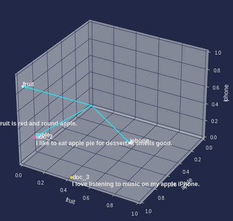
   comp_1_label = 'comp_1'
   comp_2_label = 'comp_2'
   comp_3_label = 'comp_3'
   
   fig = plt.figure(figsize=(8,8))
   ax = fig.add_subplot(projection='3d')
   
   target_words = ['apple', 'fruit', 'iphone']
   df_targets = df_comps.loc[target_words]
   df_targets = df_targets.round(5)
   df_targets = df_targets.drop_duplicates()
   
   for word, word_vec in df_targets.iterrows():
     comp_1 = word_vec[comp_1_label] * 3
     comp_2 = word_vec[comp_2_label] * 3
     comp_3 = word_vec[comp_3_label] * 3
     vec_len = np.linalg.norm(np.array([x, y, z]))
     ax.quiver(0,0,0,comp_1, comp_2, comp_3, arrow_length_ratio=0.03/vec_len)
     ax.text((comp_1+0.1), comp_2, comp_3, s=word, size=12, fontweight='bold')
     ax.scatter(comp_1, comp_2, comp_3, c='white')
   
   docs_origin_pos = df_words[target_words]
   for i, doc_pos in docs_origin_pos.iterrows():
     # 선형 변환
       x, y, z = doc_pos.dot(df_targets)
       if i=='doc_1':
               text_loc = ((x+0.1), y, (z))
       if i=='doc_2':
           text_loc = ((x+0.1), y, (z-0.1))
       if i=='doc_3':
           text_loc = ((x-0.1), y, (z-0.5))
       ax.text(*text_loc, 
               s=f'{i}\n{doc_dict[i]}',
               size=12,
               fontweight='bold')
       
       ax.scatter(x,y,z)
       
   
   ax.set_xlim(0,3)
   ax.set_ylim(3,0)
   ax.set_zlim(0,3)
   
   ax.set_xlabel(x_label, fontsize=12)
   ax.set_ylabel(y_label, fontsize=12)
   ax.set_zlabel(z_label, fontsize=12)
   
   ax.axis('off')
   
   plt.show()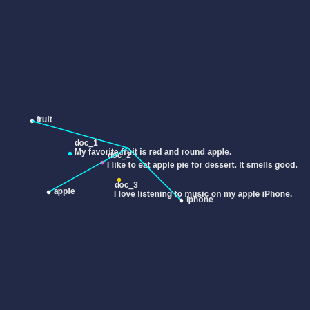

   

3-4. 문장 벡터간 유사도 계산

마지막으로, 선형 변환시킨 문장 벡터의 코사인 거리가 어떻게 바뀌었는지 확인해보겠습니다.

docs_origin_pos
>>>

df_doc_trans_pos = docs_origin_pos.dot(df_targets)
df_doc_trans_pos
>>>

dst_trans_1_2 = np.linalg.norm(df_doc_trans_pos.loc['doc_1'] - df_doc_trans_pos.loc['doc_2'])
dst_trans_2_3 = np.linalg.norm(df_doc_trans_pos.loc['doc_2'] - df_doc_trans_pos.loc['doc_3'])

cos_dst_trans_1_2 = get_cos_dst(df_doc_trans_pos.loc['doc_1'],
                               df_doc_trans_pos.loc['doc_2'])
cos_dst_trans_2_3 = get_cos_dst(df_doc_trans_pos.loc['doc_2'],
                               df_doc_trans_pos.loc['doc_3'])

print('='*20)
print(f"doc_1 : {doc_dict['doc_1']}")
print(f"doc_2 : {doc_dict['doc_2']}")
print(f"euclidean distance: {round(dst_trans_1_2,2)}")
print(f"cosine distance: {round(cos_dst_trans_1_2,2)}")

print('='*20)
print(f"doc_2 : {doc_dict['doc_2']}")
print(f"doc_3 : {doc_dict['doc_3']}")
print(f"euclidean distance: {round(dst_trans_2_3,2)}")
print(f"cosine distance: {round(cos_dst_trans_2_3,2)}")

결과)

====================
doc_1 : My favorite fruit is red and round apple.
doc_2 : I like to eat apple pie for dessert. It smells good.
**euclidean distance: 0.6
cosine distance: 0.12**
====================
doc_2 : I like to eat apple pie for dessert. It smells good.
doc_3 : I love listening to music on my apple iPhone.
**euclidean distance: 0.62
cosine distance: 0.23**

최종 결과를 확인해보면, doc_1과 doc_2의 유클리디안 거리는 0.6, 코사인 거리는 0.12 이고, doc_2과 doc_3의 유클리디안 거리는 0.62, 코사인 거리는 0.23 임을 확인할 수 있습니다.

이를 통해 doc_1과 doc_2의 유사도가 doc_2와 doc_3의 유사도보다 큼을 알 수 있었습니다.