여러 모델을 구현하고 튜닝하면서 문법적인 실력이 많이 늘었다. 아직 부족한 게 많은 건 사실이지만, 그래도 이제 머신러닝의 전반적인 진행 순서가 머릿속에 그려진다. 불과 3주 만에 다른 사람이 된 것 같다.

학습시간 09:00~02:00(당일17H/누적278H)

◆ 오늘의 깨달음

• 그리드 서치 시 estimator=XGBClassifier 부분에 estimator=는 안 적어도 된다.

search = GridSearchCV(
    XGBClassifier(
        use_label_encoder=False,
        eval_metric='logloss',
        random_state=42
    ),
    param_grid=params,
    scoring='recall',
    cv=3,
    verbose=1,
    n_jobs=-1
).fit(X_train, y_train)

• 그리드 서치로 나온 튜닝값을 **변수명.best_params_ 로 모델 안에 넣어주면 자동으로 언패킹된다. 완전 꿀팁이다.

m_xgb = XGBClassifier(
    **search.best_params_,
    random_state=42
).fit(X_train, y_train)

• 모델의 verbose와 그리드 서치의 verbose는 넣는 숫자가 다르다!! 명심!!!

LGBMClassifier(verbose=-1) 경고 메시지 숨김	
GridSearchCV(verbose=1)	진행 메시지 숨김

• classification_report 안에 정확도가 있어서 따로 accuracy_score 지표를 호출할 필요가 없다.

◆ 학습내용

예금 가입자 예측 모델 구현 2탄

3. 모델 구현

어제에 이어서

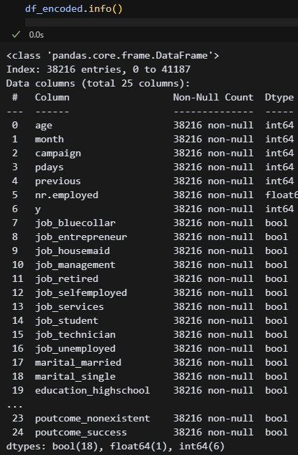
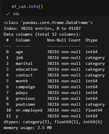어제 df를 2개로 나누는 것까지 했다. df_encoded는 원핫인코딩, df_cat는 카테고리화한 df다. CatBoost랑 LightGBM에는 카테고리 타입을 자동으로 변환하는 기능이 있다고 하는데, 과연 어떤 차이가 있을지 궁금하다.

X = df_encoded.drop(columns=['y'])
y = df_encoded['y']

일단 이녀석부터 시작해 보자! 결정트리와 앙상블기법을 사용하라고 했으니, 일단 결정트리부터 해봐야겠다. 근데 모델 이름만 보았을 때 랜덤포레스트나 캣부스트가 성능이 좋을 것 같다. 아마도...?

(1) Decision Tree

''' 모델 구현 '''
# 결정트리
from sklearn.model_selection import train_test_split
X = df_encoded.drop(columns=['y'])
y = df_encoded['y']
X_train, X_test, y_train, y_test = train_test_split(X, y, test_size=0.2, random_state=42)

from sklearn.tree import DecisionTreeClassifier
m_dtree = DecisionTreeClassifier(
    criterion = 'gini',
    min_samples_split = 3,
    min_samples_leaf = 3,
    max_features = None,
    max_depth = 5,
    max_leaf_nodes = None,
    random_state = 42
).fit(X_train, y_train)
y_train_pred = m_dtree.predict(X_train)
y_test_pred = m_dtree.predict(X_test)

from sklearn.metrics import accuracy_score, confusion_matrix, classification_report
print("▶ Train set metrics")
print("Accuracy:", accuracy_score(y_train, y_train_pred))
print("Confusion Matrix:\n", confusion_matrix(y_train, y_train_pred))
print("Classification Report:\n", classification_report(y_train, y_train_pred))
print("▶ Test set metrics")
print("Accuracy:", accuracy_score(y_test, y_test_pred))
print("Confusion Matrix:\n", confusion_matrix(y_test, y_test_pred))
print("Classification Report:\n", classification_report(y_test, y_test_pred))

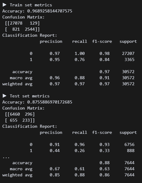
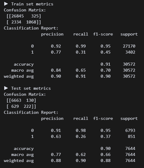
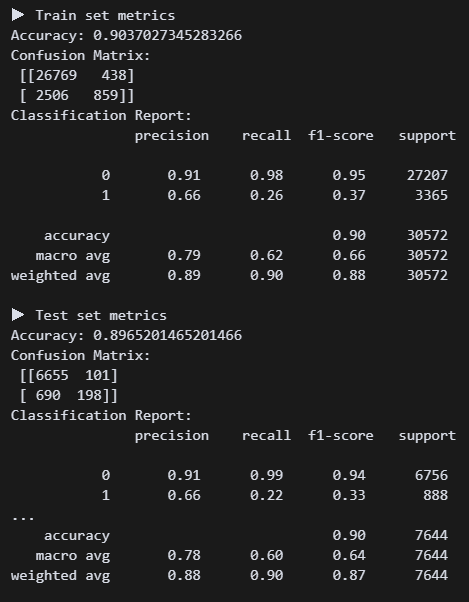결정트리 모델 구현 결과. 정확도는 괜찮은데 가입자를 못 맞추고 있다. 리콜 점수가 0.22다 ㅠㅠ 튜닝하면 괜찮아지려나?

from sklearn.model_selection import GridSearchCV
param_grid = {
    'max_depth': [3, 5, 7],
    'min_samples_split': [5, 10],
    'min_samples_leaf': [2, 5],
    'class_weight': [None, 'balanced']
}

grid = GridSearchCV(
    DecisionTreeClassifier(random_state=42),
    param_grid,
    scoring='recall',
    cv=5
).fit(X_train, y_train)

print("Best params:", grid.best_params_)
print("Best score:", grid.best_score_)

튜닝 결과가 나왔다.

m_dtree = DecisionTreeClassifier(
    class_weight = 'balanced',
    criterion = 'gini',
    min_samples_split = 5,
    min_samples_leaf = 5,
    max_features = None,
    max_depth = 5,
    max_leaf_nodes = None,
    random_state = 42
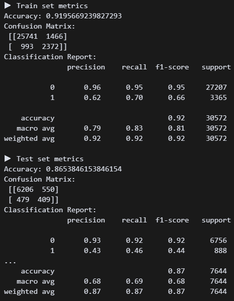
).fit(X_train, y_train)

바로 반영!
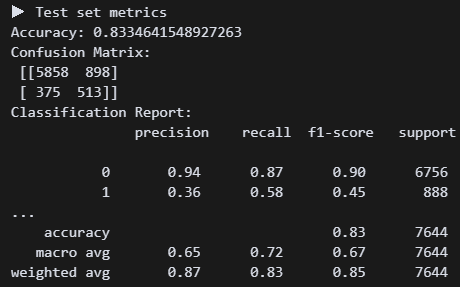오! 튜닝하니 리콜점수가 0.58로 올랐다. 정확도는 조금 낮아졌지만, 그래도 미가입자보다 가입자를 잡는 게 더 우선 아닐까?

# 시각화
import matplotlib.pyplot as plt
importances = m_dtree.feature_importances_
feat_series = pd.Series(importances, index=X.columns).sort_values(ascending=False)
plt.figure(figsize=(10, 2))
feat_series.plot(kind='bar')
plt.title('Feature Importance (Decision Tree)')
plt.ylabel('Importance Score')
plt.show()

from sklearn.tree import plot_tree
plt.figure(figsize=(20, 8))
plot_tree(m_dtree, filled=True, feature_names=X.columns)
plt.show()

어떤 요소를 기준으로 보았는지 확인해 보자!
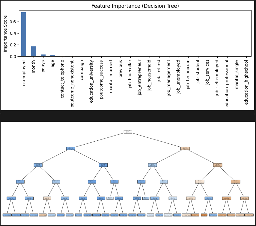고용률이 엄청 영향이 크다. 직업은 생각보다 의미가 없네.

(2) Voting

# 모델 구현
from sklearn.ensemble import VotingClassifier
from sklearn.linear_model import LogisticRegression
from sklearn.tree import DecisionTreeClassifier
from sklearn.ensemble import RandomForestClassifier

m_v1logr = LogisticRegression(max_iter=1000, class_weight='balanced', random_state=42)
m_v2tree = DecisionTreeClassifier(max_depth=5, class_weight='balanced', random_state=42)
m_v3forest = RandomForestClassifier(n_estimators=100, class_weight='balanced', random_state=42)

m_voting = VotingClassifier(
    estimators = [
        ('LOGR', m_v1logr),
        ('TREE', m_v2tree),
        ('FOREST', m_v3forest)
        ],voting = 'soft'
).fit(X_train, y_train)
y_train_pred = m_voting.predict(X_train)
y_test_pred = m_voting.predict(X_test)

from sklearn.metrics import accuracy_score, confusion_matrix, classification_report
print("▶ Train set metrics")
print("Accuracy:", accuracy_score(y_train, y_train_pred))
print("Confusion Matrix:\n", confusion_matrix(y_train, y_train_pred))
print("Classification Report:\n", classification_report(y_train, y_train_pred))
print("▶ Test set metrics")
print("Accuracy:", accuracy_score(y_test, y_test_pred))
print("Confusion Matrix:\n", confusion_matrix(y_test, y_test_pred))
print("Classification Report:\n", classification_report(y_test, y_test_pred))

보팅 모델을 구현했다. logr+tree+forest가 대표적인 조합이라고 한다.
튜닝 전인데 리콜점수가 결정트리보다 좋다. 튜닝 3개를 언제 하지 ㅠㅠ

# 튜닝(LogisticRegression)
from sklearn.model_selection import GridSearchCV
param_grid_logr = {
    'C': [0.01, 0.1, 1, 10],
    'penalty': ['l2'],
    'class_weight': ['balanced']
}
grid_logr = GridSearchCV(
    LogisticRegression(max_iter=1000, solver='lbfgs', random_state=42),
    param_grid_logr,
    scoring='recall',
    cv=3, verbose=0, n_jobs=-1
).fit(X_train, y_train)
print("Best LogisticRegression:", grid_logr.best_params_)


# 튜닝(DecisionTreeClassifier)
param_grid_tree = {
    'max_depth': [3, 5, 7],
    'min_samples_leaf': [1, 5, 10],
    'class_weight': ['balanced']
}
grid_tree = GridSearchCV(
    DecisionTreeClassifier(random_state=42),
    param_grid_tree,
    scoring='recall',
    cv=3, verbose=0, n_jobs=-1
).fit(X_train, y_train)
print("Best DecisionTree:", grid_tree.best_params_)


# 튜닝(RandomForestClassifier)
param_grid_forest = {
    'n_estimators': [100, 200],
    'max_depth': [5, 10, None],
    'max_features': ['sqrt', 'log2'],
    'class_weight': ['balanced']
}
grid_forest = GridSearchCV(
    RandomForestClassifier(random_state=42),
    param_grid_forest,
    scoring='recall',
    cv=3, verbose=0, n_jobs=-1
).fit(X_train, y_train)
print("Best RandomForest:", grid_forest.best_params_)

헉헉,,, 이렇게 하면 되는 건가...
일단 최적의 조합이 나온 것 같다. 이대로 해보자.

m_v1logr = LogisticRegression(
    C=0.01, 
    class_weight='balanced', 
    penalty=12, 
    random_state=42
)
m_v2tree = DecisionTreeClassifier(
    class_weight='balanced', 
    max_depth=5, 
    min_samples_leaf=10, 
    random_state=42
)
m_v3forest = RandomForestClassifier(
    class_weight='balanced', 
    max_depth=5, 
    max_features='sqrt'
    n_estimators=200, 
    random_state=42
)

제발!!!
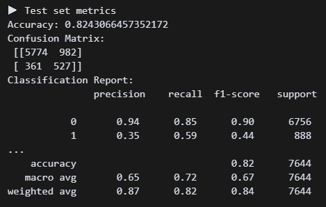오 0.59가 나왔다. 근데 결정트리랑 큰 차이가 없네.

# 차트화
import pandas as pd
m_v1logr.fit(X_train, y_train)
m_v2tree.fit(X_train, y_train)
m_v3forest.fit(X_train, y_train)

logr_importance = pd.Series(m_v1logr.coef_[0], index=X.columns)
tree_importance = pd.Series(m_v2tree.feature_importances_, index=X.columns)
forest_importance = pd.Series(m_v3forest.feature_importances_, index=X.columns)

importance_df = pd.DataFrame({
    'LogisticRegression': logr_importance,
    'DecisionTree': tree_importance,
    'RandomForest': forest_importance
})
importance_df['Avg'] = importance_df.mean(axis=1)
importance_df = importance_df.sort_values(by='Avg', ascending=False).head(10)

print("\n▶ Feature Importance \n")
print(importance_df.round(4))

3개 모델 중요도를 차트로 만들어봤다.
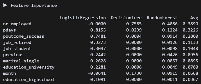고용률, 연락한 적 있는 사람, 은퇴자, 학생이 영향이 큰 것으로 보인다.

(2) Begging

''' Bagging '''
# 모델 구현
from sklearn.ensemble import RandomForestClassifier
m_forest = RandomForestClassifier(
    random_state=42,
    n_jobs=-1
).fit(X_train, y_train)
y_train_pred = m_forest.predict(X_train)
y_test_pred = m_forest.predict(X_test)

# 평가
print_metrics()

배깅의 대표모델 랜덤포레스트로 간다!(사실 다른 모델 모름)
튜닝 성능좀 보려고 하이퍼 파라미터를 아무것도 안 넣었다. 리콜수치가 0.26이다.

# 튜닝
from sklearn.model_selection import RandomizedSearchCV
params = {
    'n_estimators': [100, 200, 300],
    'max_depth': [5, 10, 20, None],
    'min_samples_split': [2, 5, 10],
    'min_samples_leaf': [1, 3, 5],
    'max_features': ['sqrt', 'log2'],
    'class_weight': ['balanced'],
    'bootstrap': [True, False]
}
search = RandomizedSearchCV(
    RandomForestClassifier(random_state=42, n_jobs=-1),
    param_distributions=params,
    n_iter=30,
    scoring='recall',
    cv=3,
    verbose=1,
    random_state=42,
    n_jobs=-1
).fit(X_train, y_train)
print("Best RandomForestClassifier:", search.best_params_)

그리드서치 20분 넘게 걸려서 랜덤서치로 변경했다. 나온 값을 넣어보자!

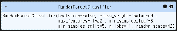
# 모델 구현
from sklearn.ensemble import RandomForestClassifier
m_forest = RandomForestClassifier(
    bootstrap=False, 
    class_weight='balanced',
    max_features='log2', 
    min_samples_leaf=5,
    min_samples_split=5, 
    n_jobs=-1, 
    random_state=42
).fit(X_train, y_train)
y_train_pred = m_forest.predict(X_train)
y_test_pred = m_forest.predict(X_test)

과연!?
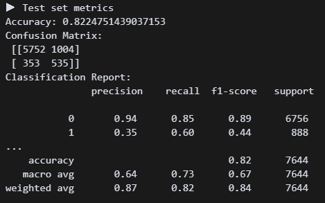와우! 정확도는 약간 떨어졌지만 리콜이 0.6으로 올라갔다.

# 시각화
importances = m_forest.feature_importances_
feat_series = pd.Series(importances, index=X.columns).sort_values(ascending=False)
plt.figure(figsize=(10, 5))
feat_series.head(10).sort_values().plot(kind='barh')
plt.title('Top 10 Feature Importance (Random Forest)')
plt.xlabel('Importance Score')
plt.tight_layout()
plt.show()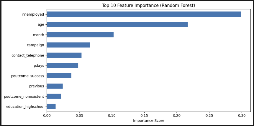

중요도 상위 10개를 봤다. 고용률, 나이, 월 순서로 중요하다. 트리도 보고 싶긴 한데, 결정 트리처럼 하나만 있는 게 아니라 모든 트리를 한 번에 볼 수 없다고 한다. 아쉽다.

# 임계값 조정
from sklearn.metrics import confusion_matrix
from sklearn.metrics import classification_report
y_proba_forest = m_forest.predict_proba(X_test)[:, 1]
threshold = 0.4
y_pred_custom = (y_proba_forest >= threshold).astype(int)
print(f"▶ RandomForest Threshold {threshold} Evaluation")
print("Confusion Matrix:\n", confusion_matrix(y_test, y_pred_custom))
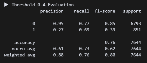
print("Classification Report:\n", classification_report(y_test, y_pred_custom))

이건 지선생이 추천해줘서 해본 건데, 아직 무슨 코드인지 정확히 이해할 수 없다. 임계값을 낮춰 내가 원하는 요소를 조금 더 잘 찾도록 하는 것 같다. threshold = 0.4 으로 했다.
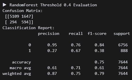정확도는 더 낮아졌지만 리콜 수치가 0.07 상승했다. 나는 미가입자를 찾는 것보다 가입자를 찾는 게 더 중요하다고 판단했다. 그래서 리콜 수치를 높여주는 이 방식이 맞는 것 같다. 일단 임계치 코드는 저장해놨다가 나중에 써봐야지!

(3) XGBoost

''' Boosting(XGBoost) '''
# 모델 구현
from xgboost import XGBClassifier
m_xgb = XGBClassifier(
    random_state=42
).fit(X_train, y_train)
y_train_pred = m_xgb.predict(X_train)
y_test_pred = m_xgb.predict(X_test)


# 평가
print_metrics()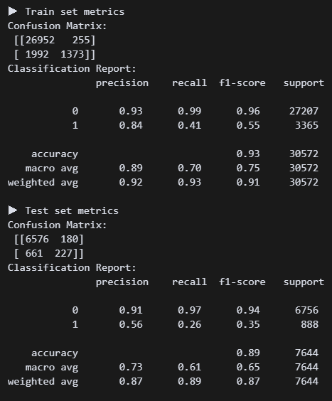

명성이 자자한 XGB. 튜닝 전후 비교를 위해 하파는 깡통으로 진행. 현재 리콜 0.26이다. 처참하군..

# 튜닝
from sklearn.model_selection import GridSearchCV
params = {
    'n_estimators': [100, 200],
    'max_depth': [3, 5, 7],
    'learning_rate': [0.05, 0.1],
    'min_child_weight': [1, 5],
    'gamma': [0, 1],
    'subsample': [0.8],
    'colsample_bytree': [0.8],
    'scale_pos_weight': [3, 5]
}
search = GridSearchCV(
    XGBClassifier(
        use_label_encoder=False,
        eval_metric='logloss',
        random_state=42
    ),
    param_grid=params,
    scoring='recall',
    cv=3,
    verbose=1,
    n_jobs=-1
).fit(X_train, y_train)
print("Best XGBClassifier:", search.best_params_)

튜닝을 해준다. 하파명이 랜포랑 비슷한 것 같긴 한데 뭔가 넣을 게 더 많은 것 같기도 하고...ㅠㅠ

Best XGBClassifier: {'colsample_bytree': 0.8, 'gamma': 1, 'learning_rate': 0.1, 'max_depth': 3, 'min_child_weight': 5, 'n_estimators': 100, 'scale_pos_weight': 5, 'subsample': 0.8} 이런 수치가 나왔다.

# 모델 재구현
from xgboost import XGBClassifier
m_xgb = XGBClassifier(
    **search.best_params_,
    use_label_encoder=False,
    eval_metric='logloss',
    random_state=42
).fit(X_train, y_train)
y_train_pred = m_xgb.predict(X_train)
y_test_pred = m_xgb.predict(X_test)
print_metrics()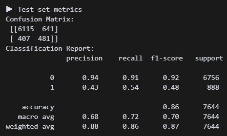

다시 해보니까 리콜 수치가 0.54로 올랐다. 왠지 랜포가 더 쉽고 좋은 것 같다. (사실 내가 튜닝을 제대로 못해서 그럼)

(4) LightGBM

''' Boosting(LightGBM)'''

# 정답 컬럼
y = df_cat['y']
X = df_cat.drop(columns=['y'])
from sklearn.model_selection import train_test_split
X_train, X_test, y_train, y_test = train_test_split(X, y, test_size=0.2, stratify=y, random_state=42)
from lightgbm import LGBMClassifier

이 녀석을 위해 어제 df를 df_encoded와 df_cat으로 나눴었다. lightBGM은 카테고리형을 자동변환해서 잡는다는데 기대가 된다.

# 모델 구현
m_lgb = LGBMClassifier(
    class_weight='balanced',
    random_state=42
).fit(X_train, y_train)
y_train_pred = m_lgb.predict(X_train)
y_test_pred = m_lgb.predict(X_test)

print_metrics()

일단 최대한 깡통으로 진행해보자.
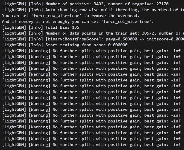뭔 경고가 엄청나게 뜬다. verbose=-1 한 줄 넣어주면 안 뜬다고 한다.

흠.. 리콜 수치가 처참하다. 튜닝튜닝튜닝!!!

# 튜닝
from sklearn.model_selection import GridSearchCV
param_grid = {
    'n_estimators': [100, 200],
    'learning_rate': [0.05, 0.1],
    'max_depth': [3, 5],
    'num_leaves': [15, 31],
    'min_child_samples': [20, 50],
    'class_weight': ['balanced']
}
grid_lgb = GridSearchCV(
    LGBMClassifier(random_state=42),
    param_grid=param_grid,
    scoring='recall',
    cv=3,
    verbose=1,
    n_jobs=-1
).fit(X_train, y_train)
best_lgb = grid_lgb.best_estimator_
print("Best LGBMClassifier:", grid_lgb.best_params_)

Best LGBMClassifier: {'class_weight': 'balanced', 'learning_rate': 0.05, 'max_depth': 3, 'min_child_samples': 20, 'n_estimators': 200, 'num_leaves': 15} 이렇게 나왔다. 바로 모델에 넣어주자!

m_lgb = LGBMClassifier(
    n_estimators=200,
    learning_rate=0.05,
    max_depth=3,
    min_child_samples=20,
    num_leaves=15,
    class_weight='balanced',
    random_state=42
).fit(X_train, y_train)
y_train_pred = m_lgb.predict(X_train)
y_test_pred = m_lgb.predict(X_test)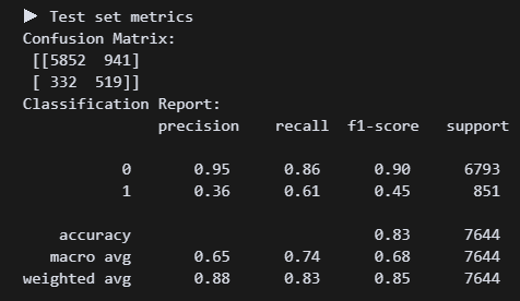

헉 0.61!???

# 임계값 조정
y_proba = m_lgb.predict_proba(X_test)[:, 1]
y_pred_custom = (y_proba >= 0.4).astype(int)
print("▶ Threshold 0.4 Evaluation")
print(classification_report(y_test, y_pred_custom))

이건 임계값도 조정해 보자!
와 0.69면 지금까지 만든 모델 중에서 베스트다....

# 시각화
import matplotlib.pyplot as plt
feat_imp = pd.Series(m_lgb.feature_importances_, index=X.columns)
top_feat = feat_imp.sort_values(ascending=False).head(10)
plt.figure(figsize=(10, 5))
top_feat.sort_values().plot(kind='barh')
plt.title("LightGBM Top 10 Feature Importance")
plt.xlabel("Importance Score")
plt.tight_layout()
plt.show()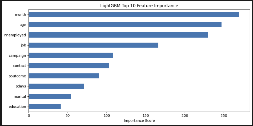

LGBM은 특이하게도 월>나이>고용률>직업 순으로 중요하게 생각했다. 음 나도 pdays나 campaign보다는 이게 맞는 방향인 것 같다.

(5) Catboost

라이브러리 설치가 안 된다 ㅠㅠ 카테고리 전문가처럼 보이는 이 녀석을 꼭 사용해 보고 싶었는데...

(6) Stacking

이 기법은 아직 이해를 제대로 못했다.. 나중에 다시 돌아오마..

4. 마치며

(1) 중요한 특성 순위

(LightGBM 모델 예측 결과 기반)

중요도 순위	변수명
1. month	마지막 연락 월
2. age	나이
3. nr.employed	고용자 수(경제 지표)
4. job	고객의 직업군
5. campaign	이번 캠페인 연락 횟수
6. contact	연락 방식
7. poutcome	이전 캠페인 결과
8. pdays	이전 연락 후 경과일
9. marital	혼인 여부
10. education	교육 수준

(2) 마케팅 전략

A. 캠페인 타이밍 전략

• month 중요도 1위 → 특정 월에 가입률이 집중됨
• 월별 성과 분석을 통해 성수기를 파악하고 성과 높은 월에 집중적인 마케팅 집행
• 3, 9, 10, 12월월 집중 캠페인 → 성과 2배”

B. 연령 기반 타겟팅

• age 중요도 2위 → 나이에 따라 가입 행동 다름
• 20대 초반 60대 이후 연령 집중적으로 캠페인 진행

C. 경제 지표 기반 시기 예측

• nr.employed 중요도 3위
• 고용률이 높을수록 고객의 여유 자금 가능성 ↑
• 외부 지표와 연동하여 타이밍 판단
• 고용자 수 증가 시점에 예금 프로모션 강화

D. 직업군별 맞춤 전략

• job 중요도 4위
• 가입률 높은 직업군 파악하여 직업군별 전용 메시지/상품 제안
• "전문직 고객을 위한 프리미엄 예금" 등

E. 연락 방식과 빈도 최적화

• contact, campaign, pdays는 “언제, 어떻게, 몇 번 연락했는가”에 관한 변수
• 너무 자주 연락하면 가입률 떨어짐 (캠페인 효율성 저하)