학습이 끝난 모델의 일부를 내가 사용할 수 있다니,, 인공지능의 세계는 알면 알수록 신기하다.

학습시간 09:00~02:00(당일17H/누적547H)

---

◆ 오늘의 깨달음

전이학습은 아래 코드가 핵심인 것 같다.

for name, param in model.named_parameters():
    if name.startswith('features'):
        param.requires_grad = False
    # print(f"{name}: {param.requires_grad}")

---

---

◆ 학습내용

1. 새로운 함수

(1) 데이터셋 정보 종합 출력

def print_dataset_info(name, train_set, test_set):
    sample_img, sample_label = train_set[0]
    print("Train 샘플 개수:", len(train_set))
    print("Test 샘플 개수:", len(test_set))

    print("샘플 이미지 텐서 shape:", sample_img.shape)
    if hasattr(train_set, 'classes'):
        print("클래스 개수:", len(train_set.classes))
        print("클래스 이름:", train_set.classes)
    print()

print_dataset_info("CIFAR100", cifar_train, cifar_test)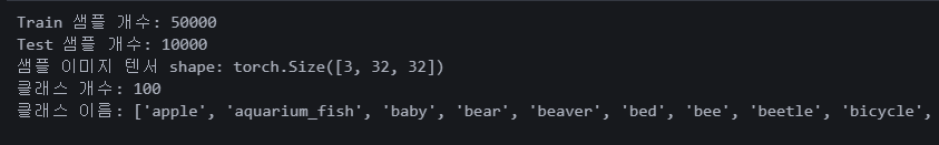

필요한 정보가 한 번에 나온다. 두고두고 써먹기 좋은 함수.

(2) 시각화 함수 1

def imshow(img, title = None, cmap = None):
    npimg = img.numpy()
    if npimg.shape[0] == 1:
        npimg = npimg[0]
    else:
        npimg = np.transpose(npimg, (1, 2, 0))
    plt.imshow(npimg, cmap = cmap)
    if title:
        plt.title(title)
    plt.axis('off')

뭔지 잘 모르겠다

(3) 시각화 함수 2

def visualize_one_per_category(dataset, dataset_name = "Dataset", cmap = None):
    samples = {}
    targets = dataset.targets if hasattr(dataset, 'targets') else dataset.train_labels

    for idx in range(len(dataset)):
        img, label = dataset[idx]

        if torch.is_tensor(label):
            label = label.item()
        if label not in samples:
            samples[label] = img
        if len(samples) >= len(dataset.classes):
            break

    n_categories = len(dataset.classes)
    print(f"{dataset_name} 카테고리 개수: {n_categories}")

    # Grid 배치를 위해 (예: 10열로 배치)
    cols = 10 if n_categories >= 10 else n_categories
    rows = math.ceil(n_categories / cols)

    fig, axes = plt.subplots(rows, cols, figsize=(cols * 2, rows * 2))
    # axes가 2차원 배열인 경우 flatten하여 사용
    if rows * cols > 1:
        axes = axes.flatten()
    else:
        axes = [axes]

    # 클래스 id 오름차순으로 정렬하여 시각화
    for i, label in enumerate(sorted(samples.keys())):
        ax = axes[i]
        img = samples[label]
        npimg = img.numpy()
        if npimg.shape[0] == 1:  # 흑백 이미지
            npimg = npimg[0]
            ax.imshow(npimg, cmap=cmap)
        else:
            npimg = np.transpose(npimg, (1, 2, 0))
            ax.imshow(npimg)
        class_name = dataset.classes[label] if hasattr(dataset, 'classes') else str(label)
        ax.set_title(class_name, fontsize=8)
        ax.axis('off')

    # 남은 subplot 축 숨기기 (있을 경우)
    for j in range(i + 1, len(axes)):
        axes[j].axis('off')

    plt.suptitle(f"{dataset_name} - 1 sample per category", fontsize=14)
    plt.tight_layout()
    plt.show()
    

모든 클래스 이미지를 한 장씩 출력하는 함수.

---

2. AlexNet 전이학습

from torchvision import models

alexnet_model = models.alexnet(weights = 'AlexNet_Weights.IMAGENET1K_V1')

이렇게 하면 모델이 다운로드 된다.
링크를 타고 들어가면 아예 pth 다운로드 가능

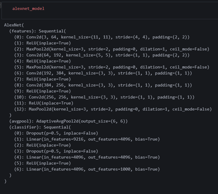알렉스넷 지정한 변수를 찍으면 __init__ 부분이 나오는 것 같다. 즉, 내가 모델을 만들진 않았지만 모델의 내부를 볼 수 있다는 뜻.

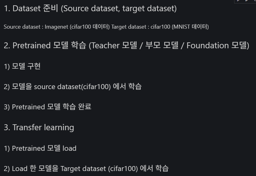전이학습 순서.

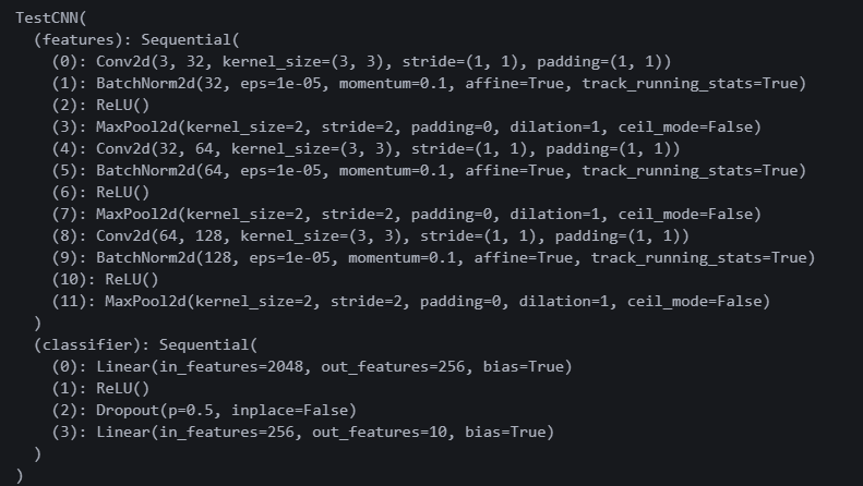적용할 모델을 수동으로 만든다.

model_cifar_dict = torch.load('./model_cifar100.pth', map_location = device)
pretrained_dict = {k:v for k, v in model_cifar_dict.items() if k.startswith('features')}

model_mnist2_dict.update(pretrained_dict)

model_mnist2.load_state_dict(model_mnist2_dict)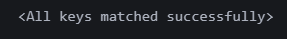

모델에 적용한다.

for param in model_mnist2.features.parameters():
    param.requires_grad = False

이렇게 특정 부분 학습을 할 것인지 정해준다.

loss_sum = 0.0
correct = 0
total = 0
num_epochs = 3
for epoch in range(num_epochs): 
    for inputs, labels in tqdm(mnist_train_loader, leave=False, desc='Train'):
        inputs, labels = inputs.to(device), labels.to(device)
        output = model_mnist2(inputs)
        loss = loss_fn(output, labels)
        loss.backward()
        optimizer_mnist2.step()
        optimizer_mnist2.zero_grad()
    
        loss_sum += loss.item() * inputs.size(0)
        _, preds = torch.max(output, 1)
        
        correct += (preds == labels).sum().item()
        total += labels.size(0)
    
    epoch_loss = loss_sum / total
    epoch_acc = correct  / total

    print(f"Epoch {epoch+1}/{num_epochs}, epoch loss : {epoch_loss}, epoch acc : {epoch_acc}")

학습을 돌려주면

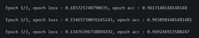정확도가 높게 나온다.

for name, param in model_mnist2.named_parameters():
    print(f"{name}: {param.requires_grad}")

이걸 하면 각 파라미터별로 학습여부가 나온다고 한다.

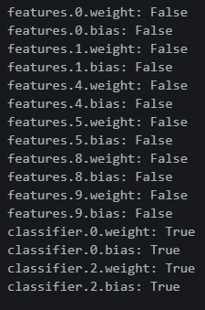이렇게!

for name, param in model_mnist2.named_parameters():
    if name.startswith('features.4.bias'):
        param.requires_grad = False
    # print(f"{name}: {param.requires_grad}")

이걸 하면 features.4. 으로 시작하는 파라미터를 조작할 수 있다.

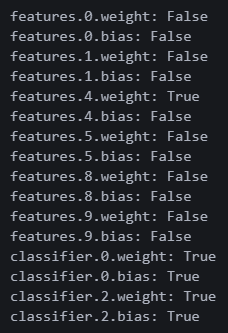4번 웨이트가 True로 변경되었다.

---

3. 전이학습 연습

(1) AlexNet 다운로드

import torchvision.models as models

alexnet = models.alexnet(pretrained=True)
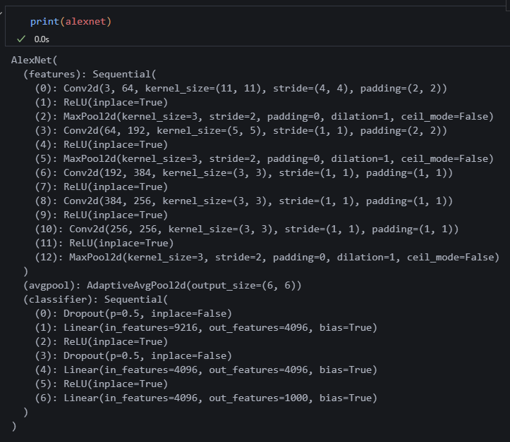
print(alexnet)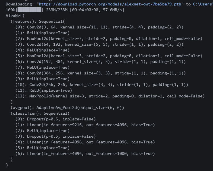

알렉스넷 다운로드 했다. features가 0~12까지 있다.

0, 3, 6, 8, 10번이 Conv2d니까 저기 웨이트가 있을 것 같다.

(2) 프리징 할 부분 선택

for name, param in alexnet.named_parameters():
    if name.startswith('features'):
        param.requires_grad = False
    print(f"{name}: {param.requires_grad}")

alexnet = alexnet.to(device)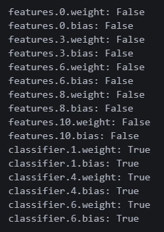

예상대로 0, 3, 6, 8, 10번 웨이트가 있다.

startswith('features') 와 requires_grad = False 를 이용해 features에 속하는 부분을 재학습되지 않도록 프리즈한다.

★ True인 부분만 학습 ★

(3) 데이터 로드

# 데이터 전처리
transform = v2.Compose([
    v2.Resize((224, 224)),  # AlexNet은 입력 224x224
    v2.ToImage(),           # PIL.Image -> torch.Tensor로 바꿔주는 과정
    v2.ToDtype(torch.float32, scale=True),  # float32로 변환 + 0~1 스케일링
    v2.Normalize(mean=[0.485, 0.456, 0.406],  # Imagenet 통계
                 std=[0.229, 0.224, 0.225]),
])

# 학습 데이터셋 로드
train_dataset = datasets.CIFAR10(root='/data', train=True, download=False, transform=transform)
train_loader = DataLoader(train_dataset, batch_size=64, shuffle=True)

데이터를 불러왔다. 알렉스넷에서 명시한 정규화 수치를 그대로 가져왔다. 간단한 CIFAR10으로 전이학습 해보자!

(4) Teacher 모델 커스텀

classifier를 보면 아웃풋이 1000이다.

(6): Linear(in_features=4096, out_features=1000, bias=True)

여기서 out_features만 수정하면 될 것 같다.

# classifier 마지막 레이어 수정 (출력 크기 10으로)
alexnet.classifier[6] = nn.Linear(4096, 10)

# 다시 디바이스로 이동 (수정했으니까)
alexnet = alexnet.to(device)

CIFAR10은 분류해야 할 클래스가 10개다. 그래서 (4096, 1000)에서 (4096, 10)으로 수정했다.

★ 수정 후에는 반드시 device!!! ★

(5) 옵티마이저 재설정

# 분류기(classifier) 파라미터만 optimizer에 전달
optimizer_new = optim.Adam(alexnet.classifier.parameters(), lr=0.001)

# CrossEntropyLoss (다중 클래스 분류 문제니까)
criterion = nn.CrossEntropyLoss()

alexnet 모델의 classifier 부분만 학습하는 것으로 옵티마이저를 수정했다.

원래 학습루프 그대로 사용하면 모델을 처음부터 다시 학습하게 된다. 그럼 Teacher 모델을 불러온 의미가 사라지니 조심해야 한다.

원래 모델명.parameters() 이렇게 쓰니까, 모델명.classifier.parameters() 이렇게 쓰면 된다.

(6) Student 모델 학습

epochs = 5

for epoch in range(epochs):
    alexnet.train()
    total_loss = 0.0

    for images, labels in tqdm(train_loader):
        images, labels = images.to(device), labels.to(device)

        # 1. optimizer 초기화
        optimizer_new.zero_grad()
        # 2. 순전파(forward)
        outputs = alexnet(images)
        # 3. 손실 계산
        loss = criterion(outputs, labels)
        # 4. 역전파(backward)
        loss.backward()
        # 5. 가중치 업데이트
        optimizer_new.step()

        total_loss += loss.item()
    print(f"Epoch [{epoch+1}/{epochs}], Loss: {total_loss/len(train_loader):.4f}")

아주 간단한 학습 코드를 만들었다.

강사님은 '백스텝제로' 순서로 하던데 대부분 '제로백스텝'이나 '제로아로백스텝' 으로 하는 것 같다. 흠,, 기능상 문제는 없나 보다.

여기서 중요한 건 학습 루프에 새로 선언한 옵티마이저 변수를 넣는 것이다. 꼭 더블 체크해야한다.

AlexNet 채널 수를 그대로 사용했더니 1에폭 돌리는데 9분이 걸린다... 저걸 기다릴 시간은 없으니 그냥 여기까지 공부한 걸로 만족하자.

---

---

이번 주도 무사히 끝!! 빨리 실습에 전이학습을 적용해 보고 싶다. 진짜 신기하다...!