ONNX의 위대함을 깨달았다.
학습시간 09:00~02:00(당일17H/누적1894H)
◆ 학습내용
모델 배포 실습
어제에 이어 4번 부터 시작!
4. 새로운 ipynb 생성
어제 코드는 modeling.ipynb에 저장했다. 오늘 코드는 inference.ipynb 파일을 새로 만들어서 넣어야 한다.
""" 데이터 로더 함수 """
def get_dataloader(batch_size):
    transform = transforms.Compose([
        transforms.ToTensor(),
        transforms.Normalize((0.5,), (0.5,))
    ])

    train_dataset = datasets.MNIST(root='./data', train=True, download=True, transform=transform)
    test_dataset = datasets.MNIST(root='./data', train=False, download=True, transform=transform)

    train_loader = DataLoader(train_dataset, batch_size=batch_size, shuffle=True)
    test_loader = DataLoader(test_dataset, batch_size=batch_size, shuffle=False)

    return train_loader, test_loader

train_loader, test_loader = get_dataloader(batch_size=64)


""" 모델 클래스 """
class SimpleCNN(nn.Module):
    def __init__(self):
        super().__init__()
        self.layer1 = nn.Sequential(
            nn.Conv2d(1, 16, 3, 1, 1),
            nn.ReLU(),
            nn.MaxPool2d(2, 2),
        )
        self.layer2 = nn.Sequential(
            nn.Conv2d(16, 32, 3, 1, 1),
            nn.ReLU(),
            nn.MaxPool2d(2, 2),
        )
        self.fc = nn.Linear(32*7*7, 10)

    def forward(self, x):
        x = self.layer1(x)
        x = self.layer2(x)
        x = x.view(-1, 32*7*7)
        x = self.fc(x)
        return x

model = SimpleCNN()
추론에 필요한 데이터와 가중치를 넣을 깡통 모델 코드다.
딱히 변경할 건 없어서 modeling.ipynb 파일에 있던 코드를 그대로 복붙했다.
5. 모델 로드 및 추론
""" PyTorch 모델 테스트 함수 """
def test_pytorch_model(model, test_loader):
    model.eval()
    correct = 0
    total = 0
    start_time = time.time()
    with torch.no_grad():
        for images, labels in test_loader:
            outputs = model(images)
            _, predicted = torch.max(outputs.data, 1)
            total += labels.size(0)
            correct += (predicted == labels).sum().item()
    end_time = time.time()
    accuracy = 100 * correct / total
    total_time = end_time - start_time
    return accuracy, total_time


""" ONNX 모델 테스트 함수 """
def test_onnx_model(ort_session, test_loader):
    correct = 0
    total = 0
    input_name = ort_session.get_inputs()[0].name
    start_time = time.time()
    for images, labels in test_loader:
        images_np = images.numpy()
        ort_inputs = {input_name: images_np}
        ort_outs = ort_session.run(None, ort_inputs)
        predicted = np.argmax(ort_outs[0], axis=1)
        total += labels.size(0)
        correct += (predicted == labels.numpy()).sum()
    end_time = time.time()
    accuracy = 100 * correct / total
    total_time = end_time - start_time
    return accuracy, total_time
로드한 가중치를 사용할 테스트 함수를 만들었다. 이 함수로 정확도와 추론 속도를 계산 할 수 있다.
근데 pth 파일과 onnx 파일의 테스트 코드가 약간 다르다. 패키지 차이로 인해 어쩔 수 없는 문제인 것 같다.
FILE_NAME = 'model'
results = {}

# .pt 모델 성능 측정
base_model = SimpleCNN()
base_model.load_state_dict(torch.load(f'{FILE_NAME}.pt'))
acc, infer_time = test_pytorch_model(base_model, test_loader)
results['Standard (.pt)'] = (acc, infer_time)

# .pth (양자화) 모델 성능 측정
quantized_model_to_load = SimpleCNN()
quantized_model = torch.quantization.quantize_dynamic(
    quantized_model_to_load, {nn.Linear, nn.Conv2d}, dtype=torch.qint8
)
quantized_model.load_state_dict(torch.load(f'{FILE_NAME}.pth'))
acc, infer_time = test_pytorch_model(quantized_model, test_loader)
results['Quantized (.pth)'] = (acc, infer_time)

# .onnx 모델 성능 측정
ort_session = onnxruntime.InferenceSession(f'{FILE_NAME}.onnx')
acc, infer_time = test_onnx_model(ort_session, test_loader)
results['ONNX (.onnx)'] = (acc, infer_time)


for name, (acc, infer_time) in results.items():
    print(f"{name} | {acc:7.2f} % | {infer_time:7.3f} seconds")
모델을 로드해서 아까 만들었던 함수로 정확도와 추론속도를 계산해준다.
pth 파일은 torch.load, onnx 파일은 onnxruntime.InferenceSession을 통해 로드 가능하다.
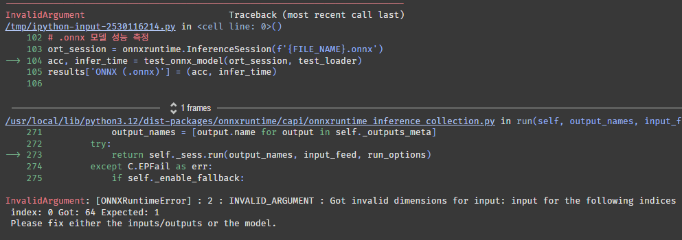
에러가 떴다. 1이 들어올 자리에 64가 들어왔다고 한다.
onnx 파일을 저장할 때 1, 1, 28, 28(B, C, H, W)로 저장했는데 이게 문제가 된 것 같다. 채널을 변경한 적은 없으니 배치 사이즈의 문제일 것 같다.
데이터로더의 배치가 64인데 이걸 1로 바꾸면 실행될까?
train_loader, test_loader = get_dataloader(batch_size=1)변경하고 다시 실행시켜보자.
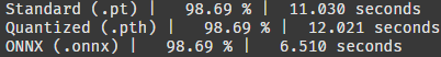
배치를 1로 하니까 동작한다! 3개 파일 모두 추론이 잘 된다.
근데 내가 원하는 건 배치사이즈에 관계없이 추론을 하는 건데 방법이 없을까?
    # ONNX 저장
    dummy_input = torch.randn(1, 1, 28, 28)  # B, C, H, W
    onnx_path = f'{file_name}.onnx'
    torch.onnx.export(
        model,
        dummy_input,
        onnx_path,
        verbose=False,
        input_names=['input'],
        output_names=['output'],
        dynamic_axes={'input' : {0 : 'batch_size'}, 'output' : {0 : 'batch_size'}}
    )
modeling.ipynb 파일에서 onnx 저장하는 코드를 약간 변경했다. dynamic_axes 파라미터를 넣어주면 된다고 한다.
아래와 같은 로그가 나왔다.
/tmp/ipython-input-2113170565.py:26: DeprecationWarning: You are using the legacy TorchScript-based ONNX export. Starting in PyTorch 2.9, the new torch.export-based ONNX exporter will be the default. To switch now, set dynamo=True in torch.onnx.export. This new exporter supports features like exporting LLMs with DynamicCache. We encourage you to try it and share feedback to help improve the experience. Learn more about the new export logic: https://pytorch.org/docs/stable/onnx_dynamo.html. For exporting control flow: https://pytorch.org/tutorials/beginner/onnx/export_control_flow_model_to_onnx_tutorial.html. torch.onnx.export( model.onnx Save Complete
이 저장 방식이 추후에 사라진다고 한다. 흠 뭐 당장은 상관 없으려나?
train_loader, test_loader = get_dataloader(batch_size=64)다시 inference.ipynb 파일로 돌아와서 배치를 64로 변경해주고,
for name, (acc, infer_time) in results.items():
    print(f"{name} | {acc:7.2f} % | {infer_time:7.3f} seconds")
실행시켜본다. 과연?
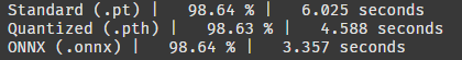
오! 작동한다! 신기하게 배치를 높이니까 양자화된 pth 파일의 추론속도가 pt 파일을 추월했다. onnx 파일 추론 속도는 여전히 가장 빠르다.
train_loader, test_loader = get_dataloader(batch_size=1024)

for name, (acc, infer_time) in results.items():
    print(f"{name} | {acc:7.2f} % | {infer_time:7.3f} seconds")
배치를 1024로 변경하고 다시 해보자
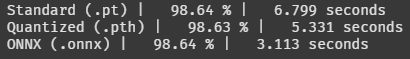
여전히 pt < pth < onnx 순이다.
정확도는 거기서 거기인듯! 그럼 onnx 파일을 사용하는 게 시간 측면에서 가장 효율적이라는 뜻이다.
근데 보기가 안 좋네. DataFrame 형식으로 바꿔야겠다.
import pandas as pd

data_for_df = []
for name, (acc, infer_time) in results.items():
    data_for_df.append({
        'Model': name,
        'Acc(%)': f"{acc:.2f}",
        'Time(s)': f"{infer_time:.3f}"
    })
df = pd.DataFrame(data_for_df)
df.index = df.index + 1
display(df)
판다스로 간단한 차트를 만들자.
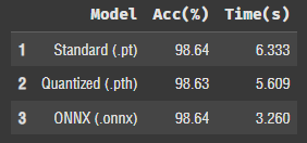
보기좋군!
근데 추론 속도가 추론할 때마다 조금씩 달라지는 것 같다.
어쨌든 onnx는 불변의 진리다.
6. TypeScript 추론
파이썬으로 만든 onnx 파일이 다른 프로그래밍 언어에서도 동일하게 작동하는지 테스트할 차례다.
요즘 핫한 타입스크립트로 해보자!
import base64
import json
import io
from IPython.display import display, HTML
from torchvision.transforms.functional import to_pil_image
from PIL import Image

# Python에서 데이터 준비
test_dataset = test_loader.dataset
prepared_data = []
for i in range(1000):
    image_tensor, label = test_dataset[i]
    pil_image = to_pil_image(image_tensor * 0.5 + 0.5)
    buffer = io.BytesIO()
    pil_image.save(buffer, format='PNG')
    image_base64 = base64.b64encode(buffer.getvalue()).decode('utf-8')
    image_data_for_ts = image_tensor.flatten().tolist()
    prepared_data.append({
        "image_base64": image_base64,
        "image_data": image_data_for_ts,
        "actual_label": label
    })
all_data_json = json.dumps(prepared_data)

with open('model.onnx', 'rb') as f:
    onnx_model_base64 = base64.b64encode(f.read()).decode('utf-8')
추론을 위한 코드다. base64, HTML 패키지를 이용하면 코랩에서 자바스크립트 기반 언어를 사용할 수 있는 듯하다. 신기하구만..!
# TypeScript + HTML 코드 작성
ts_html_code = f"""
<style>
    .inference-container {{ display: flex; flex-wrap: wrap; font-family: sans-serif; }}
    .inference-item {{ margin: 10px; padding: 10px; border: 1px solid #ccc; border-radius: 8px; text-align: center; }}
    .result {{ font-size: 1.5em; font-weight: bold; }}
    .correct {{ color: green; }}
    .incorrect {{ color: red; }}
</style>

<h3>TypeScript ONNX 추론 결과 (5개 이미지)</h3>
<div id="results-container" class="inference-container"></div>

<hr>
<div id="summary-container" style="font-family: sans-serif; margin-top: 10px;">
    <h3>📊 성능 요약</h3>
...
...
...
            // 4. 요약 정보 업데이트
            summaryDiv.innerHTML = `
                <b>정확도:</b> ${'{accuracy.toFixed(2)}'}% (${'{correctCount}'}/${'{allImageData.length}'})<br>
                <b>총 추론 시간:</b> ${'{totalTimeMs.toFixed(2)}'} ms<br>
                <b>이미지당 평균 시간:</b> ${'{avgTimeMs.toFixed(2)}'} ms
            `;

        }} catch (e) {{
            container.innerHTML = "<h2>에러 발생!</h2><p>" + e.message + "</p>";
            summaryDiv.innerText = "오류로 인해 측정 불가";
            console.error("TypeScript 에러:", e);
        }}
    }}
    runOnnxInTS();
</script>
생각보다 긴 코드가 나왔다. 과연 결과는 어떨까!?
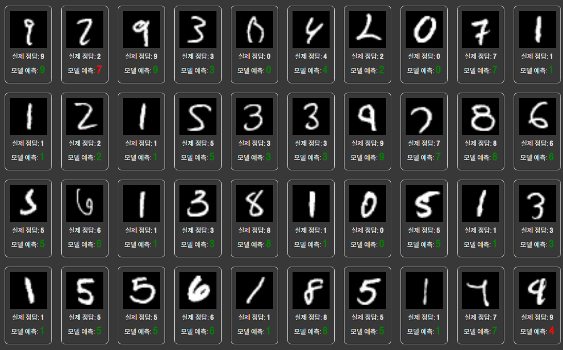
결과가 나왔다. TypeScript를 사용하니까 출력도 예쁘게 나오네 싱기방기...
사람이 봐도 헷갈릴 것 같은 이미지를 제외하곤 다 맞춘 것 같다.
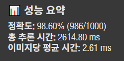
이미지 1000개 추론에 2.6초 걸렸다. 정확도도 파이썬으로 실행했던 것과 비슷하다.
즉, ONNX 파일로 변환하면 다른 프로그래밍 언어 혹은 다른 프레임워크에서 추론해도 동일한 결과가 나온다는 것이다. 속도도 빠르고 호환성도 좋고 대박이다.
ONNX 파일을 qint8 타입으로 양자화하는 방법도 있다고 하던데 나중에 다시 해봐야겠다.
결론: ONNX 최고