Input feature 늘려서 LSTM

이번에도 LSTM

저번에도 lstm으로 똑같이 삼성전자 주가를 다룬 것 아니냐고 corny하다는 이야기가 나올 수도 있음에도 불구하고 이것 또한 해보고 싶어서 한다.
흔히들 반도체, 2차 전지, Magnificent Seven과 같이 묶어서 주가를 바라보는 것에 익숙할 것이다. 이렇게 종목으로 묶을 수 있는 주식들 중에 영향을 서로 많이 준다면, correlation이 유의미하게 크다면? 과연 input feature로 넣었을 경우에 유의미한 결과를 가져올 수 있을지에 대한 의문에서 시작해서 이번 코딩을 시작했다.
코딩을 짜던 당시에 가장 핫하고 신나게 널뛰기를 하던 주식 NVDA와 SMCI를 슬쩍 비교해 보았다.

NVDA와 SMCI corr 계산

# Merge the two dataframes based on Date and focus on Adjusted Close prices
merged_df = pd.merge(nvda_df[['Date', 'Adj Close']], smci_df[['Date', 'Adj Close']], on='Date', suffixes=('_NVDA', '_SMCI'))

# Calculate the correlation between the Adjusted Close prices of NVDA and SMCI
correlation = merged_df['Adj Close_NVDA'].corr(merged_df['Adj Close_SMCI'])
correlation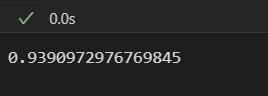

😮놀랍게도 이렇게나 높고 아름다운 숫자가 바로 나와서 사용하기로 냅다 결정했다. Adj Close(조정 종가)의 값만 비교했지만 충분하다고 생각했다 ㅎㅎ

코딩

import numpy as np

# Function to calculate RSI
def compute_rsi(data, window=14):
    delta = data.diff()
    gain = (delta.where(delta > 0, 0)).rolling(window=window).mean()
    loss = (-delta.where(delta < 0, 0)).rolling(window=window).mean()

    rs = gain / loss
    rsi = 100 - (100 / (1 + rs))
    return rsi

# Function to calculate MACD
def compute_macd(data, short_window=12, long_window=26, signal_window=9):
    short_ema = data.ewm(span=short_window, adjust=False).mean() # Short term EMA
    long_ema = data.ewm(span=long_window, adjust=False).mean() # Long term EMA
    macd = short_ema - long_ema
    signal_line = macd.ewm(span=signal_window, adjust=False).mean()
    return macd, signal_line

# Load the data
nvda_data = pd.read_csv('NVDA 주소')
smci_data = pd.read_csv('SMCI 주소')

# Calculate RSI for both datasets
nvda_data['RSI'] = compute_rsi(nvda_data['Adj Close'])
smci_data['RSI'] = compute_rsi(smci_data['Adj Close'])

# Calculate MACD for both datasets
nvda_data['MACD'], nvda_data['Signal_Line'] = compute_macd(nvda_data['Adj Close'])
smci_data['MACD'], smci_data['Signal_Line'] = compute_macd(smci_data['Adj Close'])

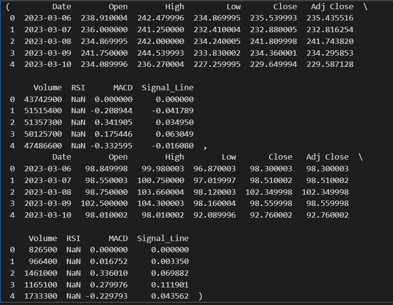
# Check the first few rows to ensure calculations are correct
nvda_data.head(), smci_data.head()

#지금 nan값으로 되어있는 것들 채워야 training 가능

그렇다고 무작정 nvda와 smci의 앞선 분석과 똑같이 feature 값만 넣는 것은 재미없으니까, 이번에는 RSI, Signal Line, MACD도 추가해서 사용하기로 했다. 주가 분석을 할 때 사용하는 가장 기본적인 추세선이기도 하니까 ㅎㅎ

추세선 종류	특징
RSI(Relative Strength Index)	- 과매수(70이상), 과매도(30이하) 상태를 식별하는데 사용되는 모멘텀 - RS = 각 거래일 종가 기준 상승분 평균/ 하락분 평균(14일 기준) - RSI = 100 - (100/1+RS)
MACD(Mobing Average Convergence Divergence	- 자산의 추세 강도와 방향, 반전을 포착하기 위한 추세선 - 12일 지수 이동평균(EMA)에서 26일 지수 이동평균을 빼서 계산
Signal Line	- MACD의 9일 지수 이동 평균을 계산하여 사용

MACD와 Signal Line 해석
MACD Line이 Signal Line을 상향 돌파하면 매수 신호
MACD Line이 Signal Line을 하향 돌파하면 매도 신호
EMA 계산하기
$EMA_t = Price_t * alpha + EMA_y * (1-alpha)$
t = today, y = yesterday
여기서 alpha = 2 / (N+1)로 MACD에서는 N=12, Signal Line에서 N=9
지금 와서 보니 추세선이 보여주는 의미를 데이터로 표현할 수 없는데...왜 넣었을까 후회가 된다 하하 그래도 training 과정에서 알아서 관계를 학습했을거라 믿어본다.

# Forward fill NaN values in the 'RSI', 'MACD', and 'Signal_Line' columns for both datasets
nvda_data[['RSI', 'MACD', 'Signal_Line']] = nvda_data[['RSI', 'MACD', 'Signal_Line']].fillna(method='ffill')
smci_data[['RSI', 'MACD', 'Signal_Line']] = smci_data[['RSI', 'MACD', 'Signal_Line']].fillna(method='ffill')

# It's possible the very first row(s) still contain NaN if the first row was NaN,
# so we can backfill those few remaining NaN values as a final step. This ensures
# the first row is not NaN by copying the first available non-NaN value backwards.
nvda_data[['RSI', 'MACD', 'Signal_Line']] = nvda_data[['RSI', 'MACD', 'Signal_Line']].fillna(method='bfill')
smci_data[['RSI', 'MACD', 'Signal_Line']] = smci_data[['RSI', 'MACD', 'Signal_Line']].fillna(method='bfill')

각주에 담아 놓은 내용과 같이; RSI, MACD, Singnal Line은 각각 26, 12, 9번째 이후로 평균값이 나오므로 앞에 값들은 모두 forward fill 해주었다. NAN값을 모두 찾아서 채워주는 꼴로 코딩했다.
처음에 멍청하게 그냥 했다가 값 없으니까 결과가 안나오더라

from sklearn.preprocessing import MinMaxScaler

mergedfirst_data = pd.merge(smci_data, nvda_data, on='Date', suffixes=('_SMCI', '_NVDA'))
merged_numerical = mergedfirst_data.drop('Date', axis=1)
# Initialize the MinMaxScaler
scaler = MinMaxScaler()

# Normalize the numerical data
mergedfirst_norm = scaler.fit_transform(merged_numerical)

# Convert the normalized arrays back to DataFrames
mergedfirst_norm_df = pd.DataFrame(mergedfirst_norm, columns=merged_numerical.columns)

# Optionally, reattach the 'Date' column if needed for reference or further analysis
mergedfirst_norm_df['Date'] = mergedfirst_data['Date']

# Reorder the columns to have 'Date' at the front if preferred
mergedfirst_norm_df = mergedfirst_norm_df[['Date'] + [col for col in mergedfirst_norm_df.columns if col != 'Date']]

merge 순서가 조금 꼬였는데; date로 merge하고, date column drop하고 minmaxscale 진행하고, 다시 붙이고 date column 추가한 것이다.

# Re-import necessary libraries and re-define functions due to reset
import pandas as pd
import numpy as np
from sklearn.preprocessing import MinMaxScaler

# Redefine create_sequences function
def create_sequences(data, sequence_length):
    xs, ys = [], []
    for i in range(len(data) - sequence_length):
        x = data[i:(i + sequence_length), :]
        y = data[i + sequence_length, 3]  # 3 corresponds to 'Close' column after scaling
        xs.append(x)
        ys.append(y)
    return np.array(xs), np.array(ys)

features = merged_data[['Open_SMCI', 'High_SMCI','Low_SMCI', 'Close_SMCI', 'Adj Close_SMCI', 'Volume_SMCI', 'RSI_SMCI', 'MACD_SMCI', 'Signal_Line_SMCI','Open_NVDA', 'High_NVDA','Low_NVDA', 'Close_NVDA', 'Adj Close_NVDA', 'Volume_NVDA', 'RSI_NVDA', 'MACD_NVDA', 'Signal_Line_NVDA']].values

# Create 14-day input sequences from the scaled features
sequence_length = 7  # Number of days
X_multi, y_multi = create_sequences(features, sequence_length)

# Split the data into training and testing sets for the multivariate case
train_size_multi = int(len(X_multi) * 0.8)
X_train_multi, X_test_multi = X_multi[:train_size_multi], X_multi[train_size_multi:]
y_train_multi, y_test_multi = y_multi[:train_size_multi], y_multi[train_size_multi:]

# Show the shapes of the resulting datasets for the multivariate case
(X_train_multi.shape, X_test_multi.shape), (y_train_multi.shape, y_test_multi.shape)

이 코드 위에 종합적으로 merge시킨 결과를 살펴보기 위한 코드가 있는데 생략했다. merged_data = mergedfirst_norm_df가 그래서 빠졌다 ㅎㅎ
코드는 앞선 삼성주가에서 사용한 코드와 동일하다. 다른 점이 있다면, sequence_length가 7이다. 이번에는 약 250일의 주가 정보만 사용하기 때문에 sequence_length가 짧아졌다. 변동성이 매우 큰 주식이라 패턴 분석을 위해 더 짧은 sequence가 더 좋은 training 결과를 보여주었다.
아이돌 안무처럼 복잡한 동작들을 20초 단위로 끊어서 알려주면 누가 다 외우겠는가 ㅎㅎㅎ 😂

# PyTorch and LSTM model re-import and re-definition due to reset
import torch
import torch.nn as nn

# Redefine the LSTM model to handle multivariate input
class MultiFeatureStockPredictorLSTM(nn.Module):
    def __init__(self, input_size, hidden_layer_size, output_size, num_layers):
        super(MultiFeatureStockPredictorLSTM, self).__init__()
        self.hidden_layer_size = hidden_layer_size

        # Define the LSTM layer(s)
        self.lstm = nn.LSTM(input_size, hidden_layer_size, num_layers, batch_first=True)

        # Define the output layer
        self.linear = nn.Linear(hidden_layer_size, output_size)

    def forward(self, input_seq):
        # Initialize hidden and cell states
        h0 = torch.zeros(self.lstm.num_layers, input_seq.size(0), self.hidden_layer_size).to(input_seq.device)
        c0 = torch.zeros(self.lstm.num_layers, input_seq.size(0), self.hidden_layer_size).to(input_seq.device)
        
        # Get LSTM outputs
        lstm_out, _ = self.lstm(input_seq, (h0, c0))
        
        # Get the prediction from the last time step
        prediction = self.linear(lstm_out[:, -1, :])
        return prediction

# Adjusted model parameters for multivariate input
input_size = 18  
hidden_layer_size = 60  # Number of hidden units in each LSTM layer
output_size = 1  # Predicting a single 'Close' price
num_layers = 3  # Number of LSTM layers

# Initialize the adjusted model
multi_feature_model = MultiFeatureStockPredictorLSTM(input_size, hidden_layer_size, output_size, num_layers)
multi_feature_model

# Define the loss function and optimizer
loss_function = nn.MSELoss()
optimizer = torch.optim.Adam(multi_feature_model.parameters(), lr=0.001)

# Convert data to PyTorch tensors
X_train_tensors = torch.Tensor(X_train_multi)
y_train_tensors = torch.Tensor(y_train_multi).view(-1, 1)
X_test_tensors = torch.Tensor(X_test_multi)
y_test_tensors = torch.Tensor(y_test_multi).view(-1, 1)

# Set the number of epochs and initialize a variable to track the minimum test loss
num_epochs = 200
min_test_loss = np.inf

# Training loop
for epoch in range(num_epochs):
    multi_feature_model.train()
    optimizer.zero_grad()
    output = multi_feature_model(X_train_tensors)
    loss = loss_function(output, y_train_tensors)
    loss.backward()
    optimizer.step()
    
    # Evaluation on the test data
    multi_feature_model.eval()
    test_predictions = multi_feature_model(X_test_tensors)
    test_loss = loss_function(test_predictions, y_test_tensors)
    
    # Save the model if the test loss decreased
    if test_loss < min_test_loss:
        min_test_loss = test_loss
        torch.save(multi_feature_model.state_dict(), '모델 저장할 주소')  # Save the best model
    
    # Print the loss every 10 epochs
    if epoch % 50 == 0:
        print(f'Epoch {epoch+1}/{num_epochs}, Training Loss: {loss.item()}, Test Loss: {test_loss.item()}')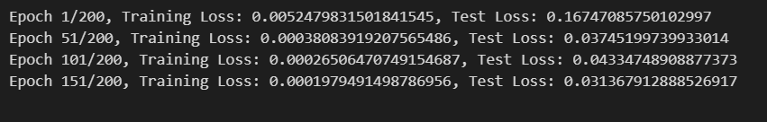

여기서 epoch을 200개로 설정했다. epoch이 뭔지 한번도 적어놓은 적이 없는 것 같아서 이야기해보자면, One Epoch: This means that every sample in the training dataset has been used once to update the model's weights. 실제 주가를 따라가는 함수를 내가 만드는 작업에서, weight를 업데이트해야(coefficent) 목표 모델에 가까워진다. 여기서 한 번의 위의 일련의 과정이 일어나면 one epoch이 되는 것이다. 우리는 이것을 200번 시킨 것이다. 여기서 어지러운 점이 epoch 수가 과도하게 많아도 Overfitting을 발생시킬 수 있다는 것이다.^^

# Load the best model
best_model_path = '위에서 저장한 베스트 모델 주소'
multi_feature_model.load_state_dict(torch.load(best_model_path))

# Make predictions with the best model
multi_feature_model.eval()  # Set the model to evaluation mode
with torch.no_grad():  # No need to track gradients
    predicted_test = multi_feature_model(X_test_tensors).cpu().numpy()

# Inverse transform the predictions and actual values to their original scale
predicted_test_prices = scaler.inverse_transform(
    np.concatenate([X_test_multi[:, -1, :3], predicted_test, X_test_multi[:, -1, 4:]], axis=1)
)[:, 3]  # Select only the 'Close' column

actual_test_prices = scaler.inverse_transform(
    np.concatenate([X_test_multi[:, -1, :3], y_test_multi.reshape(-1, 1), X_test_multi[:, -1, 4:]], axis=1)
)[:, 3]  # Select only the 'Close' column

# Plotting
import matplotlib.pyplot as plt

plt.figure(figsize=(15, 6))
plt.plot(actual_test_prices, label='Actual Close Prices', color='blue')
plt.plot(predicted_test_prices, label='Predicted Close Prices', color='red')
plt.title('Comparison of Actual and Predicted Close Prices')
plt.xlabel('Time (latest -> oldest)')
plt.ylabel('Close Price')
plt.legend()
plt.show()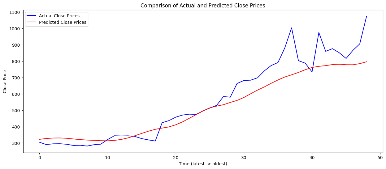

보아하니 결과는 처참?하다. 아무래도 volatility가 상당히 높다보니 LSTM이 pattern 분석하는데 한계가 있어보이긴 한다. 또한 250일 정도의 짧은 데이터로 인해 한계가 보인다. 사실 일부로 변동성이 높은 종목을 선정해서 늘어난 feature들이 패턴 분석에 도움이 얼마나 될지 알아보기 위함도 있었다. 아무래도 feature들(정말 의미 있는)도 부족하고 지켜본 기간도 아쉬웠다.
그래도 RSI, MACD, Signal Line도 계산해보고 현재까지도 재밌게 요동치고 있는 두 반도체 회사에 대해 알아본 것으로 위안을 얻는다. 다음에는 parameter 선정에 대한 논문들과 최근 어떤 데이터들을 주가 예측에 사용하는지 최신 트렌드의 논문들을 좀 읽어보고 진행해보겠다. 또한 Montecarlo simulation과 Brownian method를 사용해보는 것도 공부해보려고 한다.

Today's Quote

What question would you ask an AGI system once you create it?
(from Lex Fridman's podcast with Elon Musk)

본 내용은 누군가에게 정보를 제공하고자 작성한 글이 아니다(실력이 안됨)
본인이 공부하면서 깨달은? 내용들의 기록 용도임을 밝힌다.
무한한 피드백과 태클을 걸어도 된다. 양분으로 감사하게 받아 먹겠다.