LSTM으로 삼성전자 주가 예측

LSTM

이번에는 전 포스팅과 거의 유사하지만 RNN보다 뛰어나다고 알려진 LSTM을 이용해서 똑같이 삼성전자를 분석해보도록 하겠다.

어느 부분에서 뛰어난가?

사실 그저 뛰어나다고 해서 가져와서 시작해봤다.

Feature	RNN	LSTM
Basic Concept	form a directed graph along a temporal sequence	capable of learning long-term dependencies
Structure	single hidden layer and feedback loops	more complex structure with memory cells and multiple gates(input, output, forget)

표는 영어로 이렇게 있어 보이게 적어 보았지만,
1. LSTM이 long-term dependencies and context 부분에서 성능이 더 뛰어나다
2. LSTM은 (input, output, forget) 3가지 gates로 이루어졌지만, RNN은 single hidden layer와 feedback loops로만 이루어져있다. 즉 LSTM이 더 복잡하다.
나중에 기회가 된다면 구조에 대해서 깊게 파는 포스팅을 하겠다

코드

이번에는 RNN 때보다는 rough하게 나누어서 설명하겠다.
똑같이 삼성전자의 데이터를 사용할 것이며, column 또한 똑같다.

import pandas as pd
import numpy as np
from sklearn.preprocessing import MinMaxScaler

def create_sequences(data, sequence_length):
    xs, ys = [], []
    for i in range(len(data) - sequence_length):
        x = data[i:(i + sequence_length), :]
        y = data[i + sequence_length, 3] 
        xs.append(x)
        ys.append(y)
    return np.array(xs), np.array(ys)

# 데이터 불러오기, Scaling
file_path = '해당 주소 ㅎㅎ'
samsung_data = pd.read_csv(file_path)
features = samsung_data[['Open', 'High', 'Low', 'Close', 'Volume']].values
scaler_multi = MinMaxScaler(feature_range=(0, 1))
scaled_features = scaler_multi.fit_transform(features)

sequence_length = 60  
X_multi, y_multi = create_sequences(scaled_features, sequence_length)

# training, testing 세트 나누기
train_size_multi = int(len(X_multi) * 0.8)
X_train_multi, X_test_multi = X_multi[:train_size_multi], X_multi[train_size_multi:]
y_train_multi, y_test_multi = y_multi[:train_size_multi], y_multi[train_size_multi:]

# 데이터셋 결과 출력
(X_train_multi.shape, X_test_multi.shape), (y_train_multi.shape, y_test_multi.shape)

출력결과 = (((1125, 60, 5), (282, 60, 5)), ((1125,), (282,)))

• sequence_length = 60인 이유: LSTM은 long-term 데이터에 특화된 만큼 RNN에서 사용한 5보다는 확실히 길다. 60일은 LSTM으로 주식을 분석할때 가장 기본적인 설정으로 알려져 있다. 60일 정도가 회사의 분기 실적 발표의 영향을 분석하기 편하다는 의견도 있지만, 가장 큰 이유는 "해보니 잘돼서"가 아닐까 싶다.
• MinMaxScaler: RNN에서도 사용했으나 따로 설명을 넣지 않아서, 가볍게 적어보겠다. (0,1)의 range의 scale로 바꾸기 위한 대표적인 방법으로, (X - X_min) / (X_max - X_min)의 공식을 이용한다.
• 전체 데이터 수에서 80%를 training으로 사용하기로 정했다. 지금보니 X로 표현하지 않았다 ㅎㅎ

import torch
import torch.nn as nn

# LSTM 함수
class MultiFeatureStockPredictorLSTM(nn.Module):
    def __init__(self, input_size, hidden_layer_size, output_size, num_layers):
        super(MultiFeatureStockPredictorLSTM, self).__init__()
        self.hidden_layer_size = hidden_layer_size

        # Define the LSTM layers
        self.lstm = nn.LSTM(input_size, hidden_layer_size, num_layers, batch_first=True)

        # Define the output layer
        self.linear = nn.Linear(hidden_layer_size, output_size)

    def forward(self, input_seq):
        # Initialize hidden and cell states
        h0 = torch.zeros(self.lstm.num_layers, input_seq.size(0), self.hidden_layer_size).to(input_seq.device)
        c0 = torch.zeros(self.lstm.num_layers, input_seq.size(0), self.hidden_layer_size).to(input_seq.device)
        
        # Get LSTM outputs
        lstm_out, _ = self.lstm(input_seq, (h0, c0))
        
        # Get the prediction from the last time step
        prediction = self.linear(lstm_out[:, -1, :])
        return prediction

input_size = 5  # Number of features (Open, High, Low, Close, Volume)
hidden_layer_size = 50  # 본인 설정 가능
output_size = 1  # Predicting a single 'Close' price
num_layers = 2  # Number of LSTM layers(본인 설정 가능)

# Initialize the adjusted model
multi_feature_model = MultiFeatureStockPredictorLSTM(input_size, hidden_layer_size, output_size, num_layers)
multi_feature_model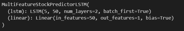

이렇게 보면 RNN과 다른 parameter가 없다.
batch_first=True is primarily about making your data easier to organize and work with.

# Define the loss function and optimizer
loss_function = nn.MSELoss()
optimizer = torch.optim.Adam(multi_feature_model.parameters(), lr=0.001)

# Convert data to PyTorch tensors
X_train_tensors = torch.Tensor(X_train_multi)
y_train_tensors = torch.Tensor(y_train_multi).view(-1, 1)
X_test_tensors = torch.Tensor(X_test_multi)
y_test_tensors = torch.Tensor(y_test_multi).view(-1, 1)

# Set the number of epochs and initialize a variable to track the minimum test loss
num_epochs = 100
min_test_loss = np.inf

# Training loop
for epoch in range(num_epochs):
    multi_feature_model.train()
    optimizer.zero_grad()
    output = multi_feature_model(X_train_tensors)
    loss = loss_function(output, y_train_tensors)
    loss.backward()
    optimizer.step()
    
    # Evaluation on the test data
    multi_feature_model.eval()
    test_predictions = multi_feature_model(X_test_tensors)
    test_loss = loss_function(test_predictions, y_test_tensors)
    
    # Save the model if the test loss decreased
    if test_loss < min_test_loss:
        min_test_loss = test_loss
        torch.save(multi_feature_model.state_dict(), '모델의 새로운 주소')  # Save the best model
    
    # Print the loss every 10 epochs
    if epoch % 10 == 0:
        print(f'Epoch {epoch+1}/{num_epochs}, Training Loss: {loss.item()}, Test Loss: {test_loss.item()}')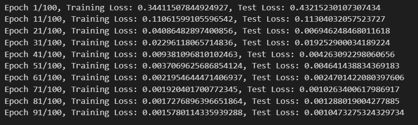

일단 MSELoss는 가장 흔한 Mean Squared Error Loss이고 RNN 때와 똑같이 parameter update는 Adam에게 맡기겠다. RNN 때와 일단 가장 큰 차이점은 훈련 epoch의 개수이다. 사실상 RNN에서의 그래프 결과만 봐도 알 수 있듯이 overfitting된 경향이 보인다. Overfitting은 training data의 training 과정에서 디테일과 노이즈들까지 과하게 훈련 받아 실제 data에 적용이 불가능한 경우를 말한다. 모의고사만 잘 풀고 수능 망하는 것이다^^.

# Load the best model
best_model_path = '모델 주소'
multi_feature_model.load_state_dict(torch.load(best_model_path))

# Make predictions with the best model
multi_feature_model.eval()  # Set the model to evaluation mode
with torch.no_grad():  # No need to track gradients
    predicted_test = multi_feature_model(X_test_tensors).cpu().numpy()

# Inverse transform the predictions and actual values to their original scale
predicted_test_prices = scaler_multi.inverse_transform(
    np.concatenate([X_test_multi[:, -1, :3], predicted_test, X_test_multi[:, -1, 4:]], axis=1)
)[:, 3]  # Select only the 'Close' column

actual_test_prices = scaler_multi.inverse_transform(
    np.concatenate([X_test_multi[:, -1, :3], y_test_multi.reshape(-1, 1), X_test_multi[:, -1, 4:]], axis=1)
)[:, 3]  # Select only the 'Close' column

# Plotting
import matplotlib.pyplot as plt

plt.figure(figsize=(15, 6))
plt.plot(actual_test_prices, label='Actual Close Prices', color='blue')
plt.plot(predicted_test_prices, label='Predicted Close Prices', color='red')
plt.title('Comparison of Actual and Predicted Close Prices')
plt.xlabel('Time (latest -> oldest)')
plt.ylabel('Close Price')
plt.legend()
plt.show()

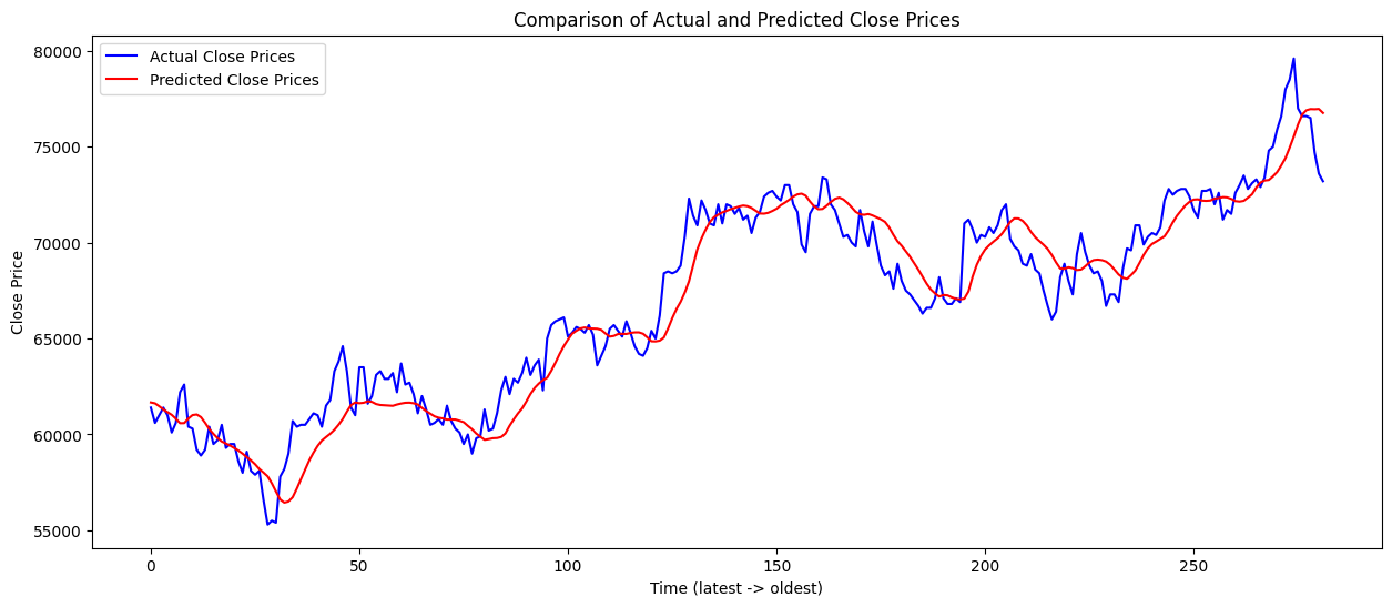
그래프의 결과는 위의 그림과 같다.
이번 미니 프로젝트에서 알아야 할 것: seqeunce_length = 60인 이유, Overfitting, RNN과 LSTM의 차이?

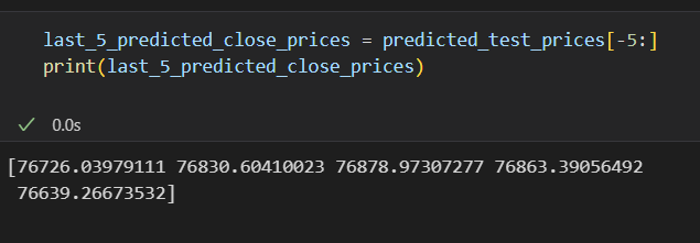
다른 포스팅들을 살펴보니, 결국 예측값은 위와 같이 마지막 5개 정도의 데이터를 뽑아서 mean을 사용하거나 마지막 gradient를 반영하여 예측하는 정도였다. 과연 이게 머신러닝을 이용한 prediction이라는 표현이 맞을까 하는 의구심이 들긴 한다. 이렇기 때문에 대부분의 금융공학의 paper들은 volatility나 identification에 집중하는 것이 아닐까 싶다.

Today's Quote

Never really harm of scaling.
("Andrew Ng" in Machine Learning Specialization)

본 내용은 누군가에게 정보를 제공하고자 작성한 글이 아니다(실력이 안됨)
본인이 공부하면서 깨달은? 내용들의 기록 용도임을 밝힌다.
무한한 피드백과 태클을 걸어도 된다. 양분으로 감사하게 받아 먹겠다.