[KT 에이블스쿨] 6차 미니프로젝트

🚗 6차 미니 프로젝트

미션: 차량 공유업체의 차량 파손 여부 분류

활용 데이터셋

자체 제작 데이터 : Car_images.zip

도메인 이해

차량공유업체에게 필요한 차량 파손 여부를 알려주는 서비스를 개발하는 것이 목표.
차량을 공유하고, 반납 시에 파손 여부를 자동화하는 것이다.

데이터 분석 및 전처리

• 모델1 전처리

# 압축 해제

data = zipfile.ZipFile(path+file1)

try :
    print('압축을 해제합니다.')
    data.extractall(path)
    print('압축 해제가 완료되었습니다.')
except :
    pass
    print('압축이 이미 해제되었거나 이미 폴더가 존재합니다.')
    
# 폴더별 이미지 데이터 갯수 확인

print(f"정상 차량 이미지 데이터는 {len(glob.glob(path+'normal/*'))}장 입니다.")
print(f"파손 차량 이미지 데이터는 {len(glob.glob(path+'abnormal/*'))}장 입니다.")

#정상 차량 이미지 데이터는 302장 입니다.
#파손 차량 이미지 데이터는 303장 입니다.
    

# Load "normal" images
normal_images = glob.glob(path + 'normal/*')
for image_path in normal_images:
    img = image.load_img(image_path, target_size=(280, 280))
    img = image.img_to_array(img)
    img = np.expand_dims(img, axis=0)
    X.append(img)


# Load "abnormal" images
abnormal_images = glob.glob(path + 'abnormal/*')
for image_path in abnormal_images:
    img = image.load_img(image_path, target_size=(280, 280))
    img = image.img_to_array(img)
    img = np.expand_dims(img, axis=0)
    X.append(img)


# Combine all images into a single numpy array
X = np.vstack(X)

print(f"총 이미지 개수: {len(X)}")

#총 이미지 개수: 605

# X와 Y 데이터를 분할
X_train, X_temp, Y_train, Y_temp = train_test_split(X, Y1, test_size=0.2, random_state=42)
X_valid, X_test, Y_valid, Y_test = train_test_split(X_temp, Y_temp, test_size=0.5, random_state=42)

# 각 데이터셋의 크기 확인
print(f"Train set 크기: {len(X_train)}")
print(f"Validation set 크기: {len(X_valid)}")
print(f"Test set 크기: {len(X_test)}")

#Train set 크기: 484
#Validation set 크기: 60
#Test set 크기: 61

• 모델2 전처리

import os
import shutil
import random

# 폴더 경로 설정
project_dir = '/content/drive/MyDrive/project/'
source_normal_dir = os.path.join(project_dir, "normal")
source_abnormal_dir = os.path.join(project_dir, "abnormal")

train_dir = os.path.join(project_dir, "Car_Images_train")
val_dir = os.path.join(project_dir, "Car_Images_val")
test_dir = os.path.join(project_dir, "Car_Images_test")

# 대상 폴더 생성
for dir_path in [train_dir, val_dir, test_dir]:
    os.makedirs(os.path.join(dir_path, "normal"), exist_ok=True)
    os.makedirs(os.path.join(dir_path, "abnormal"), exist_ok=True)

# 이미지 파일 목록 가져오기
normal_images = os.listdir(source_normal_dir)
abnormal_images = os.listdir(source_abnormal_dir)

# 이미지 무작위 섞기
random.shuffle(normal_images)
random.shuffle(abnormal_images)

# 이미지 분배 비율 설정 (8:1:1)
total_normal = len(normal_images)
total_abnormal = len(abnormal_images)

train_ratio = 0.8
val_ratio = 0.1
test_ratio = 0.1

train_normal_count = int(total_normal * train_ratio)
val_normal_count = int(total_normal * val_ratio)
test_normal_count = int(total_normal * test_ratio)

train_abnormal_count = int(total_abnormal * train_ratio)
val_abnormal_count = int(total_abnormal * val_ratio)
test_abnormal_count = int(total_abnormal * test_ratio)

# 이미지를 대상 폴더로 복사
for i in range(train_normal_count):
    image_name = normal_images[i]
    source_path = os.path.join(source_normal_dir, image_name)
    target_path = os.path.join(train_dir, "normal", image_name)
    shutil.copy(source_path, target_path)

for i in range(train_abnormal_count):
    image_name = abnormal_images[i]
    source_path = os.path.join(source_abnormal_dir, image_name)
    target_path = os.path.join(train_dir, "abnormal", image_name)
    shutil.copy(source_path, target_path)

for i in range(train_normal_count, train_normal_count + val_normal_count):
    image_name = normal_images[i]
    source_path = os.path.join(source_normal_dir, image_name)
    target_path = os.path.join(val_dir, "normal", image_name)
    shutil.copy(source_path, target_path)

for i in range(train_abnormal_count, train_abnormal_count + val_abnormal_count):
    image_name = abnormal_images[i]
    source_path = os.path.join(source_abnormal_dir, image_name)
    target_path = os.path.join(val_dir, "abnormal", image_name)
    shutil.copy(source_path, target_path)

for i in range(train_normal_count + val_normal_count, total_normal):
    image_name = normal_images[i]
    source_path = os.path.join(source_normal_dir, image_name)
    target_path = os.path.join(test_dir, "normal", image_name)
    shutil.copy(source_path, target_path)

for i in range(train_abnormal_count + val_abnormal_count, total_abnormal):
    image_name = abnormal_images[i]
    source_path = os.path.join(source_abnormal_dir, image_name)
    target_path = os.path.join(test_dir, "abnormal", image_name)
    shutil.copy(source_path, target_path)

모델링

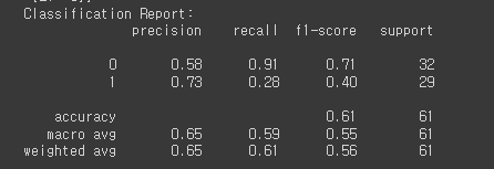
• 모델 1

model = Sequential()
model.add(Conv2D(32, (3, 3), activation='relu', input_shape=(280, 280, 3)))
model.add(MaxPool2D((2, 2)))
model.add(Conv2D(64, (3, 3), activation='relu'))
model.add(MaxPool2D((2, 2)))
model.add(Conv2D(128, (3, 3), activation='relu'))
model.add(MaxPool2D((2, 2)))
model.add(Flatten())
model.add(Dense(128, activation='relu'))
model.add(Dense(1, activation='sigmoid'))
model.compile(optimizer='adam', loss='binary_crossentropy', metrics=['accuracy'])
early_stopping = EarlyStopping(patience=5, restore_best_weights=True)

history = model.fit(X_train, Y_train, epochs=50, validation_data=(X_valid, Y_valid), callbacks=[early_stopping])

# 모델 평가
Y_pred = model.predict(X_test)
Y_pred_binary = (Y_pred > 0.5)
print("Confusion Matrix:")
print(confusion_matrix(Y_test, Y_pred_binary))
print("Classification Report:")
print(classification_report(Y_test, Y_pred_binary))

• ResNet50

import keras
from keras.applications import ResNet50
from keras.models import Sequential
from keras.layers import Dense, GlobalAveragePooling2D
from keras.callbacks import EarlyStopping
from sklearn.metrics import classification_report, confusion_matrix

# ResNet-50 모델 불러오기 (weights='imagenet'은 사전 훈련된 가중치를 사용)
base_model = ResNet50(weights='imagenet', include_top=False)

# 모델 설계
model3 = Sequential()

# ResNet-50 모델을 포함하고, Global Average Pooling 레이어를 추가
model3.add(base_model)
model3.add(GlobalAveragePooling2D())

# Fully Connected 레이어 추가
model3.add(Dense(256, activation='relu'))
model3.add(Dense(1, activation='sigmoid'))

# 모델 컴파일
model3.compile(optimizer='adam', loss='binary_crossentropy', metrics=['accuracy'])

# Early Stopping 설정
early_stopping = EarlyStopping(patience=5, restore_best_weights=True)
lr = ReduceLROnPlateau(monitor = 'val_accuracy',
                       factor = 0.1,
                       patience = 3,
                       verbose = 1,
                       mode = 'auto',
                       min_delta = 0.01,
                       min_lr = 0)
checkpoint = ModelCheckpoint("model_checkpoint.h5", save_best_only=True)

x = base_model.output
x = GlobalAveragePooling2D()(x)
x = Dense(128, activation='relu')(x)
x = Dropout(0.3)(x)
predictions = Dense(1, activation='sigmoid')(x)

resnet50 = Model(inputs=base_model.input , outputs=predictions)

resnet50.compile(loss=keras.losses.binary_crossentropy,
               metrics=['accuracy'],
               optimizer= keras.optimizers.Adam(learning_rate = 0.0001))
               
history3 = resnet50.fit(X_train, Y_train, epochs=9, validation_data=(X_valid, Y_valid), callbacks=[early_stopping,lr,checkpoint])


# 모델 평가
Y_pred = resnet50.predict(X_test)
Y_pred_binary = (Y_pred > 0.5)
print("Confusion Matrix:")
print(confusion_matrix(Y_test, Y_pred_binary))
print("Classification Report:")
print(classification_report(Y_test, Y_pred_binary))

• Data Augmentation

train_datagen = ImageDataGenerator(
    rescale=1./255,  # 이미지 픽셀값 0~255를 0~1로 정규화
    rotation_range=10,  # 이미지 회전 각도 범위
    zoom_range=0.3,  # 이미지 확대/축소 범위
    brightness_range=[0.5, 1.5],  # 이미지 명도 범위
    channel_shift_range=50,  # 이미지 채도 범위
    horizontal_flip=True,  # 수평 방향으로 이미지 뒤집기
    vertical_flip=True,  # 수직 방향으로 이미지 뒤집기
    fill_mode='nearest'  # 이미지 변환 후 빈 영역을 채우는 방법
)

valid_datagen = ImageDataGenerator(
    rescale=1./255,
)

test_datagen = ImageDataGenerator(
    rescale=1./255,
)

train_generator = train_datagen.flow_from_directory(
          train_path,
          target_size=(280, 280),
          class_mode='binary',
          shuffle = True,
          )

valid_generator = valid_datagen.flow_from_directory(
          valid_path,
          target_size=(280, 280),
          class_mode='binary',
          shuffle = True,
          )

test_generator = test_datagen.flow_from_directory(
          test_path,
          target_size=(280, 280),
          class_mode='binary',
          shuffle = False,
          )
          
          

• VGG16

from tensorflow.keras.applications import VGG16
from tensorflow.keras.models import Sequential
from tensorflow.keras.layers import Flatten, Dense

# VGG16 모델 불러오기 (사전 학습된 가중치를 포함)
base_model = VGG16(weights='imagenet', include_top=False, input_shape=(280, 280, 3))

# VGG16 모델의 가중치를 동결 (fine-tuning 전에 동결하는 것이 일반적)
for layer in base_model.layers:
    layer.trainable = False

# 새로운 분류 레이어를 추가한 모델 설계
vggmodel = Sequential()
vggmodel.add(base_model)  # VGG16 모델을 추가
vggmodel.add(Flatten())  # Flatten 레이어 추가
vggmodel.add(Dense(128, activation='relu'))  # 완전 연결(Dense) 레이어 추가
vggmodel.add(Dense(1, activation='sigmoid'))  # 이진 분류를 위한 출력 레이어 (클래스가 2개인 경우)

# 모델 컴파일
vggmodel.compile(optimizer='adam', loss='binary_crossentropy', metrics=['accuracy'])

# 모델 요약 확인
vggmodel.summary()

from tensorflow.keras.models import load_model
# Early Stopping 콜백 설정
early_stopping = EarlyStopping(monitor='val_loss', patience=5, verbose=1, restore_best_weights=True)

# ModelCheckpoint 콜백 설정 (최적 가중치 저장)
model_checkpoint = ModelCheckpoint('best_model.h5', monitor='val_loss', save_best_only=True)

lr = ReduceLROnPlateau(monitor = 'val_accuracy',
                       factor = 0.1,
                       patience = 3,
                       verbose = 1,
                       mode = 'auto',
                       min_delta = 0.01,
                       min_lr = 0)

# 모델 학습
epochs = 100  # 적절한 학습 에포크 수를 설정하세요.

history = vggmodel.fit(
    train_datagen.flow_from_directory(train_path, target_size=(280, 280), class_mode='binary', batch_size=32),
    validation_data=valid_generator,
    epochs=epochs,
    callbacks=[early_stopping, model_checkpoint,lr],  # Early Stopping 및 ModelCheckpoint 콜백 사용
    verbose=1
)

# 최적 모델 가중치를 불러옵니다.
best_model = load_model('best_model.h5')

# 최적 모델로 평가
test_loss, test_accuracy = best_model.evaluate(test_generator, verbose=1)
print(f'Test Accuracy with Best Model: {test_accuracy * 100:.2f}%')


# 테스트 데이터로 모델 평가
test_results = best_model.evaluate(test_generator, steps=test_generator.samples // test_generator.batch_size)

# 예측 결과 계산
Y_pred = best_model.predict(test_generator)
Y_pred_binary = (Y_pred > 0.5)

# 모델 평가 결과 출력
print("Test Loss:", test_results[0])
print("Test Accuracy:", test_results[1])

# Confusion Matrix 및 Classification Report 출력
print("Confusion Matrix:")
print(confusion_matrix(test_generator.classes, Y_pred_binary))
print("Classification Report:")
print(classification_report(test_generator.classes, Y_pred_binary))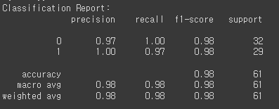

• EfficientNetV2B0

from tensorflow.keras.applications import EfficientNetV2B0
keras.backend.clear_session()

base_model = EfficientNetV2B0(weights='imagenet', include_top=False, input_shape=(280, 280,3))
base_model.trainable = True

# 새로운 분류 레이어를 추가한 모델 설계
effmodel = Sequential()
effmodel.add(base_model)  # EfficientNetV2B0 모델을 추가
effmodel.add(Flatten())  # Flatten 레이어 추가
effmodel.add(Dense(128, activation='relu'))  # 완전 연결(Dense) 레이어 추가
effmodel.add(Dense(1, activation='sigmoid'))  # 이진 분류를 위한 출력 레이어 (클래스가 2개인 경우)

# 모델 컴파일
effmodel.compile(optimizer='adam', loss='binary_crossentropy', metrics=['accuracy'])

# 모델 요약 확인
effmodel.summary()

from tensorflow.keras.models import load_model
# Early Stopping 콜백 설정
early_stopping = EarlyStopping(monitor='val_loss', patience=5, verbose=1, restore_best_weights=True)

# ModelCheckpoint 콜백 설정 (최적 가중치 저장)
model_checkpoint = ModelCheckpoint('best_model_eff.h5', monitor='val_loss', save_best_only=True)

lr = ReduceLROnPlateau(monitor = 'val_accuracy',
                       factor = 0.1,
                       patience = 3,
                       verbose = 1,
                       mode = 'auto',
                       min_delta = 0.01,
                       min_lr = 0)

# 모델 학습
epochs = 100  # 적절한 학습 에포크 수를 설정하세요.

history = effmodel.fit(
    train_datagen.flow_from_directory(train_path, target_size=(280, 280), class_mode='binary', batch_size=32),
    validation_data=valid_generator,
    epochs=epochs,
    callbacks=[early_stopping, model_checkpoint,lr],  # Early Stopping 및 ModelCheckpoint 콜백 사용
    verbose=1
)

# 최적 모델 가중치를 불러옵니다.
best_model_eff = load_model('best_model_eff.h5')

# 최적 모델로 평가
test_loss, test_accuracy = best_model_eff.evaluate(test_generator, verbose=1)
print(f'Test Accuracy with Best Model: {test_accuracy * 100:.2f}%')

# 테스트 데이터로 모델 평가
test_results = best_model_eff.evaluate(test_generator, steps=test_generator.samples // test_generator.batch_size)

# 예측 결과 계산
Y_pred = best_model_eff.predict(test_generator)
Y_pred_binary = (Y_pred > 0.5)

# 모델 평가 결과 출력
print("Test Loss:", test_results[0])
print("Test Accuracy:", test_results[1])

# Confusion Matrix 및 Classification Report 출력
print("Confusion Matrix:")
print(confusion_matrix(test_generator.classes, Y_pred_binary))
print("Classification Report:")
print(classification_report(test_generator.classes, Y_pred_binary))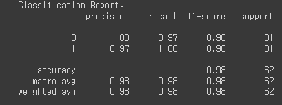

🚩6차 미니 프로젝트를 마치며
눈 깜빡하니 벌써 미프 6차다. 이번 프로젝트는 차량 파손 여부를 판별하는 주제로 진행했다. 이미지라서 그런지 학습 중에 런타임이 끊기기도 했다. 이번에 프로젝트에서도 느꼈듯이 pre-trained model을 잘 사용하는 것이 성능을 높일 수 있는 지름길이다. 미프 6차가 끝났다는 건 벌써 6개월의 교육기간 중 3개월이 지났다는 뜻! 3개월동안 성장한 부분도 있지만, 아쉬운 부분도 있다. 남은 3개월은 더 알차게 보내보자!