Pytorch
tensorflow같은 tensor를 사용하는 framework
설치conda install pytorch torchvision torchaudio cpuonly -c pytorch
새로운 가상환경을 만들어 주고, pytorch를 설치함
pytorch를 이용하여 실습을 해보자
보스턴 집 값 예측
data load
현재 load_boston은 삭제되어 사용할 수 없어서 아래 코드로 대체하였다.
EDA
import torch
import torch.nn as nn
import torch.nn.functional as F
import torch.optim as optim

#학습에 필요한 특성 선택
cols = ['INDUS', 'RM', 'LSTAT', 'NOX', 'DIS']
data_X = torch.from_numpy(X[cols].values).float()
data_y = torch.from_numpy(y.values).float()

data_X.shape
(결과) torch.Size([506, 5])

#변수 설정
X = data_X
y =  data_y.reshape(len(data_y),1)
print(X.shape, y.shape)
(결과) torch.Size([506, 5]) torch.Size([506, 1])
Modeling
#하이파라미터
n_epochs = 2000
learning_rate = 1e-3
print_interval = 100
#모델 수립
model = nn.Linear(X.size(-1), y.size(-1))
model
(결과) Linear(in_features=5, out_features=1, bias=True)
#optimizer
optimizer = optim.SGD(model.parameters(), lr=learning_rate)
#학습
for i in range(n_epochs):
y_hat = model(X)
loss = F.mse_loss(y_hat, y) #먼저 loss 계산
optimizer.zero_grad() #gradient 초기화
#역전파에서 gradient를 더해가는 것이 default인데 for문을 돌때마다 더하면 안되므로
loss.backward()
optimizer.step()
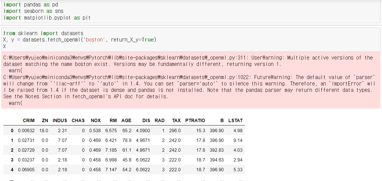
if (i+1) % print_interval == 0: #100의 배수일때 loss 표현
print('Epoch %d: loss=%.4e' % (i + 1, loss))
#결과 정리
df = pd.DataFrame(torch.cat([y, y_hat], dim=1).detach_().numpy(),
columns=['y', 'y_hat'])
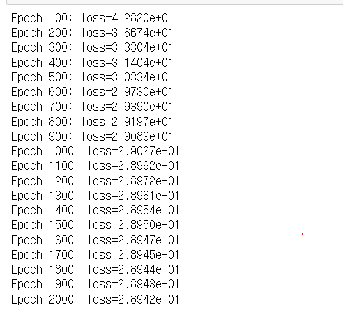
sns.pairplot(df, height=5)
plt.show() 1번째 그래프가 참값, 4번째 그래프가 예측값인데 참값에서 끝부분은 예측하지 못했다.
끝부분을 학습 시키기가 쉽지 않다는 뜻이기도 하다
Breast Cancer
data
from sklearn.datasets import load_breast_cancer
cancer = load_breast_cancer()
#print(cancer.DESCR)

import torch
import torch.nn as nn
import torch.nn.functional as F
import torch.optim as optim

data = torch.from_numpy(df[cols].values).float()

#데이터 분리
df = pd.DataFrame(cancer.data, columns=cancer.feature_names)
df['class'] = cancer.target

#컬럼 추출
cols = ['mean radius', 'mean texture', 'mean smoothness', 'mean compactness',
       'mean concave points', 'worst radius', 'worst texture', 'worst smoothness',
       'worst compactness', 'worst concave points', 'class']

for c in cols[:-1]:
    sns.histplot(df, x=c, hue=cols[-1], bins=50, stat='probability')
    plt.show()
Modeling
#하이파라미터
n_epochs = 200000
learnin_rate = 1e-2
print_interval = 10000

#model
class MyModel(nn.Module):

    def __init__(self, input_dim, output_dim):
        self.input_dim = input_dim
        self.output_dim = output_dim

        super().__init__()

        self.linear = nn.Linear(input_dim, output_dim)
        self.act = nn.Sigmoid()

    def forward(self, x):
        #|x| = (batch_size, input_dim)
        y = self.act(self.linear(x))
        #|y| = (batch_size, output_dim)

        return y

#모델, loss, optim선언
model = MyModel(input_dim=X.size(-1),output_dim=y.size(-1))
crit = nn.BCELoss() #mse 대신 BCE (Binary Cross Entropy)
optimizer = optim.SGD(model.parameters(),lr=learning_rate)

#학습
for i in range(n_epochs):
    y_hat = model(X)
    loss = crit(y_hat, y)

    optimizer.zero_grad()
    loss.backward()

    optimizer.step()

    if (i+1)%print_interval == 0:
        print('Epoch %d : loss=%.4e' % (i+1, loss))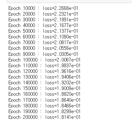
#acc계산
correct_cnt = (y == (y_hat > .5)).sum()
total_cnt = float(y.size(0))
print('Accuracy: %.4f' % (correct_cnt / total_cnt))
#Accuracy: 0.9420
#예측값 분포 확인
df = pd.DataFrame(torch.cat([y,y_hat], dim=1).detach().numpy(),
columns=['y', 'y_hat'])
sns.histplot(df, x='y_hat', hue='y', bins=50, stat='probability')
plt.show()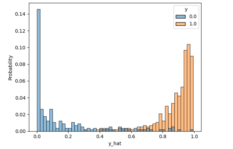
MNIST
import torch
import torch.nn as nn
import torch.nn.functional as F
import torch.optim as optim
from torchvision import datasets, transforms

from matplotlib import pyplot as plt
%matplotlib inline

#Cuda가 가능하면 cuda 아니면 cpu 설정
is_cuda = torch.cuda.is_available()
device = torch.device('cuda' if is_cuda else 'cpu')

print('Current cuda device is', device)
GPU가 사용하능 하다면, Current cuda device is cuda
아니라면, Current cuda device is cpu가 출력됨
data
#파라미터 설정
batch_size = 50
learning_rate = 0.0001
epoch_num = 15

#root='./data' : 현재 코드가 실행되는 위치에 다운
#train 옵션 : train 가능한 데이터
#download = True (처음에만 다운, 나중에는 한번 받았으니 False로 두면 됨)
#transforms.ToTensor() 바로 tensor로 바꾸는 옵션
train_data = datasets.MNIST(root='./data', train=True, download=True,
                           transform = transforms.ToTensor())
test_data = datasets.MNIST(root='./data', train=False,
                           transform = transforms.ToTensor())
print('number of training data : ', len(train_data))
print('number of test data : ', len(test_data))
number of training data : 60000
number of test data : 10000
image, label = train_data[0]

#squeeze() : 차원이 1인 것을 없애는 옵션 [1, 28, 28] -> [28,28]
plt.imshow(image.squeeze().numpy(), cmap='gray')
plt.title('label : %s' % label)
plt.show()
#keras에서는 채널의 차원이 제일 뒤에 오는데 torch에서는 제일 앞에 온다.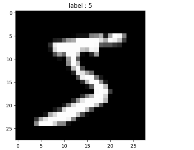
Modeling
미니 배치를 구성하여 모델링을 해본다.
이 때, 배치는 전체 데이터를 쪼개서 학습시키는 것을 말한다.
#미니 배치 구성
#shuffle : 데이터의 순서를 학습하지 못하게 한다
train_loader = torch.utils.data.DataLoader(dataset = train_data,
                                           batch_size = batch_size, shuffle=True)
test_loader = torch.utils.data.DataLoader(dataset = test_data,
                                           batch_size = batch_size, shuffle=True)
#첫번째 배치만 가져오면
first_batch = train_loader.__iter__().__next__()

# 배치 결과 확인
# {:15s} : 15칸 확보, <:좌측정렬, > : 우측정렬
print('{:15s} | {:<25s} | {}'.format('name', 'type', 'size'))
print('{:15s} | {:<25s} | {}'.format('Num of Batch', '', len(train_loader)))
print('{:15s} | {:<25s} | {}'.format('first_batch', str(type(first_batch)),
                                     len(first_batch)))
print('{:15s} | {:<25s} | {}'.format('first_batch[0]', str(type(first_batch[0])),
                                     first_batch[0].shape))
print('{:15s} | {:<25s} | {}'.format('first_batch[1]', str(type(first_batch[1])),
                                     first_batch[1].shape))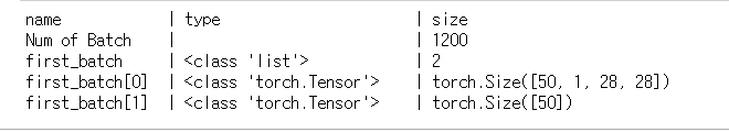
- 총 6만개 데이터가 배치로 1200개 묶음
- 첫번째 배치는 0번,1번이 있음
- 1번은 라벨인데, 50개씩 묶었기 때문에 50개
- 0번은 픽셀 데이터인데, 50개는 데이터 갯수, 채널 1, 가로 세로
#model
class CNN(nn.Module):
    def __init__(self):
        super(CNN, self).__init__()
        #nn.Conv2d(입력 채널 수, 출력 채널, 커널 사이즈, stride 수, 제로패딩옵션)
        self.conv1 = nn.Conv2d(1, 32, 3, 1, padding='same')
        self.conv2 = nn.Conv2d(32, 64, 3, 1, padding='same')
        self.dropout = nn.Dropout2d(0.25)
        self.fc1 = nn.Linear(3136, 1000) # 7*7*64 = 3136
        self.fc2 = nn.Linear(1000, 10)

    def forward(self, x):
        x = self.conv1(x) #(28,28)
        x = F.relu(x)
        x = F.max_pool2d(x, 2) #(14,14)

        x = self.conv2(x) #(14,14)
        x = F.relu(x)
        x = F.max_pool2d(x, 2) #(7,7)

        x = self.dropout(x)
        x = torch.flatten(x, 1)
        x = self.fc1(x)
        x = F.relu(x)
        x = self.fc2(x)
        output = F.log_softmax(x, dim=1)
        return output

#model
model = CNN().to(device)
optimizer = optim.Adam(model.parameters(), lr=learning_rate)
criterion = nn.CrossEntropyLoss()

#학습
model.train() #학습선언만 한것, 실제 학습은 아님
i = 1
for epoch in range(epoch_num):
    for data, target in train_loader: #미니 배치로 구성된 데이터
        data = data.to(device)
        target = target.to(device)
        optimizer.zero_grad()
        output = model(data)
        loss = criterion(output, target)
        loss.backward()
        optimizer.step()
        if i % 1000 == 0:
            print('Train Step : {}\tLoss : {:.3f}'.format(i, loss.item()))
        i +=1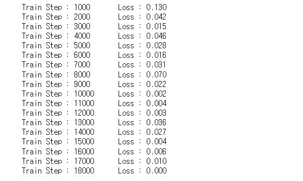
#성능 평가
model.eval() #평가 선언(dropout 기능 꺼짐)
correct = 0
for data, target in test_loader:
  data = data.to(device)
  target = target.to(device)
  output = model(data)
  prediction = output.data.max(1)[1] #argmax 기능. max값의 인덱스를 추출
  correct += prediction.eq(target.data).sum() #정답 개수를 합산


print('Test set: Accuracy: {:.2f}%'.format(100. * correct / len(test_loader.dataset)))
Test set: Accuracy: 99.15%