1. 머신러닝이란?
머신러닝(기계 학습, Machine Learning)은 컴퓨터가 명시적으로 프로그래밍되지 않아도 데이터를 통해 학습하고 예측을 할 수 있도록 하는 기술이다.
기본적으로 머신러닝은 대량의 데이터를 분석하여 패턴을 찾아내고, 그 패턴을 기반으로 미래의 데이터를 예측하거나 분류하는 데 사용된디.
머신 러닝의 주요 개념
- 데이터: 머신러닝 모델을 훈련시키기 위해서는 대량의 데이터가 필요.
이 데이터는 입력(features)과 출력(labels)으로 구성될 수 있음.
- 모델: 데이터에서 패턴을 학습하는 알고리즘.
모델은 다양한 형태를 취할 수 있으며, 학습 방식에 따라 여러 종류로 나뉨.
- 훈련(training): 모델이 주어진 데이터에서 패턴을 학습하는 과정.
모델은 데이터를 통해 가중치를 조정하고, 이를 통해 예측을 더욱 정확하게 만듬.
- 테스트(testing): 학습된 모델의 성능을 평가하는 과정.
훈련에 사용되지 않은 새로운 데이터를 사용하여 모델의 예측 능력을 검증.
- 평가(evaluation): 모델의 성능을 수치적으로 평가하는 단계.
예를 들어, 정확도(accuracy), 정밀도(precision), 재현율(recall), F1 점수 등이 사용.
머신러닝의 종류
- 지도 학습(Supervised Learning): 입력 데이터와 그에 상응하는 출력 라벨이 주어질 때, 모델이 입력 데이터를 출력에 맞추어 학습하는 방식.
예) 이미지 분류, 스팸 이메일 탐지.
- 비지도 학습(Unsupervised Learning): 입력 데이터만 주어지고, 출력 라벨이 없는 경우.
모델은 데이터의 구조나 패턴을 스스로 찾아냄.
예) 군집화(clustering)나 차원 축소(dimensionality reduction).
- 강화 학습(Reinforcement Learning): 에이전트가 환경과 상호작용하며 보상을 최대화하는 방향으로 학습하는 방.
예) 게임 플레이, 로봇 제어.
2. 회귀 분석
회귀 분석이란?
회귀분석(Regression Analysis)은 두 개 이상의 변수 간의 관계를 분석하고 모델링하는 통계 기법.
주로 하나의 종속 변수(반응 변수)와 하나 이상의 독립 변수(설명 변수) 간의 관계를 파악하고 예측하는 데 사용.
회귀분석의 목표는 주어진 독립 변수들로부터 종속 변수를 예측하는 모델을 만드는 것
1. 단순 회귀(Simple Regression)
단순 회귀는 하나의 독립 변수(x)와 하나의 종속 변수(y) 간의 관계를 직선으로 모델링하는 방법.
이 방법은 두 변수 간의 선형 관계를 분석하고 예측할 때 사용.사용상황
- 두 변수 간의 관계를 단순하게 설명하고자 할 때
- 예) 키(x)와 몸무게(y) 간의 관계를 분석할 때
2. 다항 회귀(Polynomial Regression)
다항 회귀는 독립 변수와 종속 변수 간의 비선형 관계를 모델링하기 위해 독립 변수의 다항식 항을 추가하는 방법.
이는 곡선 형태의 관계를 모델링할 때 유용.사용 상황
- 변수들 간의 관계가 비선형일 때
- 예) 차량의 속도(x)와 연료 소비량(y) 간의 관계가 비선형일 때
3. 다중 회귀(Multiple Regression)
다중 회귀는 여러 개의 독립 변수와 하나의 종속 변수 간의 관계를 모델링하는 방법.
이는 여러 변수들이 종속 변수에 미치는 영향을 동시에 분석할 때 사용.사용 상황
- 종속 변수에 영향을 미치는 여러 요인을 분석하고자 할 때
- 예) 주택 가격(y)을 방의 수(x1), 지역(x2), 건축 연도(x3) 등의 여러 변수들로 예측할 때
요약
- 단순 회귀: 두 변수 간의 선형 관계를 분석할 때 사용.
- 다항 회귀: 변수 간의 비선형 관계를 모델링할 때 사용.
- 다중 회귀: 여러 변수들이 종속 변수에 미치는 영향을 동시에 분석할 때 사용.
2-1) 단순 회귀 분석
# -*- coding: utf-8 -*-
### 기본 라이브러리 불러오기
import pandas as pd
import numpy as np
import matplotlib.pyplot as plt
import seaborn as sns

'''
[Step 1] 데이터 준비 - read_csv() 함수로 자동차 연비 데이터셋 가져오기
'''
# CSV 파일을 데이터프레임으로 변환
df = pd.read_csv('data/auto-mpg.csv', header=None)
df

### 출력 결과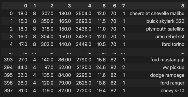
# 열 이름 지정
df.columns = ['mpg','cylinders','displacement','horsepower','weight',
              'acceleration','model year','origin','name']
속성 정보 :
1. mpg : 연속
2. 실린더 : 다중 값 이산
3. 변위 : 연속
4. 마력 : 연속
5. 무게 : 연속
6. 가속 : 연속
7. 모델 연도 : 다중 값 이산
8. 원점 : 다중 값 이산
9. 자동차 이름 : 문자열 (각 인스턴스에 대해 고유함)
# 데이터 살펴보기
df.head()

### 출력 결과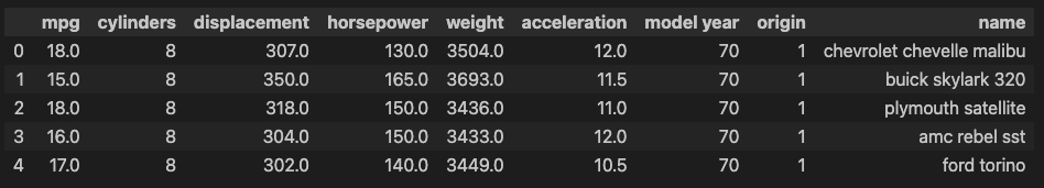
'''
[Step 2] 데이터 탐색
'''
# 데이터 자료형 확인
df.info()

### 출력 결과
<class 'pandas.core.frame.DataFrame'>
RangeIndex: 398 entries, 0 to 397
Data columns (total 9 columns):
 #   Column        Non-Null Count  Dtype
---  ------        --------------  -----
 0   mpg           398 non-null    float64
 1   cylinders     398 non-null    int64
 2   displacement  398 non-null    float64
 3   horsepower    398 non-null    object
 4   weight        398 non-null    float64
 5   acceleration  398 non-null    float64
 6   model year    398 non-null    int64
 7   origin        398 non-null    int64
 8   name          398 non-null    object
dtypes: float64(4), int64(3), object(2)
memory usage: 28.1+ KB
# 데이터 통계 요약정보 확인
df.describe()
### 출력 결과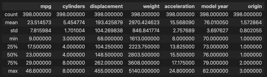
# horsepower 열의 자료형 변경 (문자열 ->숫자)
df['horsepower'].unique()          # horsepower 열의 고유값 확인

### 출력 결과
array(['130.0', '165.0', '150.0', '140.0', '198.0', '220.0', '215.0',
       '225.0', '190.0', '170.0', '160.0', '95.00', '97.00', '85.00',
       '88.00', '46.00', '87.00', '90.00', '113.0', '200.0', '210.0',
       '193.0', '?', '100.0', '105.0', '175.0', '153.0', '180.0', '110.0',
       '72.00', '86.00', '70.00', '76.00', '65.00', '69.00', '60.00',
       '80.00', '54.00', '208.0', '155.0', '112.0', '92.00', '145.0',
       '137.0', '158.0', '167.0', '94.00', '107.0', '230.0', '49.00',
       '75.00', '91.00', '122.0', '67.00', '83.00', '78.00', '52.00',
       '61.00', '93.00', '148.0', '129.0', '96.00', '71.00', '98.00',
       '115.0', '53.00', '81.00', '79.00', '120.0', '152.0', '102.0',
       '108.0', '68.00', '58.00', '149.0', '89.00', '63.00', '48.00',
       '66.00', '139.0', '103.0', '125.0', '133.0', '138.0', '135.0',
       '142.0', '77.00', '62.00', '132.0', '84.00', '64.00', '74.00',
       '116.0', '82.00'], dtype=object)

df['horsepower'].replace('?', np.nan, inplace=True)      # '?'을 np.nan으로 변경
df.dropna(subset=['horsepower'], axis=0, inplace=True) # 누락데이터 행을 삭제
df['horsepower'] = df['horsepower'].astype('float') # 문자열을 실수형으로 변환
df.describe()
### 출력 결과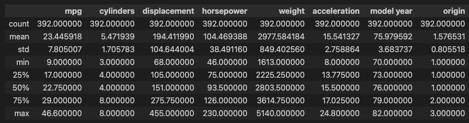
'''
[Step 3] 속성(feature 또는 variable) 선택
'''
# 분석에 활용할 열(속성)을 선택 (연비, 실린더, 출력, 중량)
ndf = df[['mpg', 'cylinders', 'horsepower', 'weight']]
ndf.head()

### 출력 결과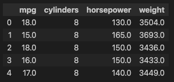
### 종속 변수 Y인 "연비(mpg)"와 다른 변수 간의 선형관계를 그래프(산점도)로 확인
# Matplotlib으로 산점도 그리기
ndf.plot(kind='scatter', x='weight', y='mpg',  c='coral', s=10, figsize=(10, 5))
plt.show()
plt.close()

### 출력 결과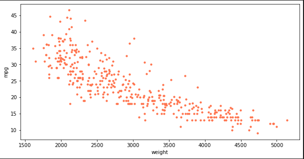
# seaborn으로 산점도 그리기
fig = plt.figure(figsize=(10, 5))
ax1 = fig.add_subplot(1, 2, 1)
ax2 = fig.add_subplot(1, 2, 2)
sns.regplot(x='weight', y='mpg', data=ndf, ax=ax1)                 # 회귀선 표시
sns.regplot(x='weight', y='mpg', data=ndf, ax=ax2, fit_reg=False)  #회귀선 미표시
plt.show()
plt.close()

### 출력 결과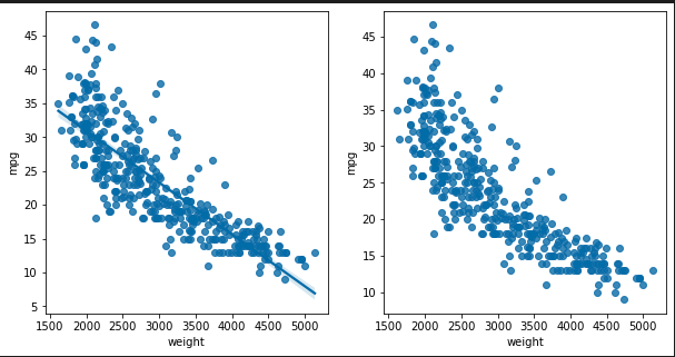
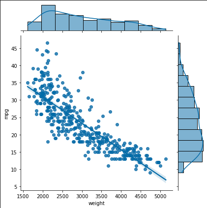
# seaborn 조인트 그래프 - 산점도, 히스토그램
sns.jointplot(x='weight', y='mpg', data=ndf)              # 회귀선 없음
sns.jointplot(x='weight', y='mpg', kind='reg', data=ndf)  # 회귀선 표시
plt.show()
plt.close()

### 출력 결과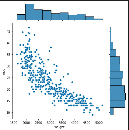
# seaborn pariplot으로 두 변수 간의 모든 경우의 수 그리기
sns.pairplot(ndf)
plt.show()
plt.close()

### 출력 결과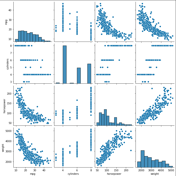
'''
Step 4: 데이터셋 구분 - 훈련용(train data)/검증용(test data)
'''
# 속성(변수) 선택
X=ndf[['weight']]  #독립 변수 X
y=ndf['mpg']       #종속 변수 Y

# train data 와 test data로 구분(7:3 비율)
from sklearn.model_selection import train_test_split
X_train, X_test, y_train, y_test = train_test_split(X,               #독립 변수
                                                    y,               #종속 변수
                                                    test_size=0.3,   #검증 30%
                                                    random_state=10) #랜덤 추출 값

print('train data 개수: ', len(X_train))
print('test data 개수: ', len(X_test))

### 출력 결과
train data 개수:  274
test data 개수:  118
'''
Step 5: 단순회귀분석 모형 - sklearn 사용
'''
# sklearn 라이브러리에서 선형회귀분석 모듈 가져오기
from sklearn.linear_model import LinearRegression
# 단순회귀분석 모형 객체 생성
lr = LinearRegression()
# train data를 가지고 모형 학습
lr.fit(X_train, y_train)
### 출력 결과
LinearRegression()
# 학습을 마친 모형에 test data를 적용하여 결정계수(R-제곱) 계산
r_square = lr.score(X_test, y_test)
print(r_square)
### 출력 결과
0.6822458558299322
# 회귀식의 기울기
print('기울기 a: ', lr.coef_)
### 출력 결과
기울기 a: [-0.00775343]
# 회귀식의 y절편
print('y절편 b', lr.intercept_)
### 출력 결과
y절편 b 46.7103662572801# 모형에 전체 X 데이터를 입력하여 예측한 값 y_hat을 실제 값 y와 비교
y_hat = lr.predict(X)
plt.figure(figsize=(10, 5))
ax1 = sns.distplot(y, hist=False, label="y") # 정답 : 파란색
ax2 = sns.distplot(y_hat, hist=False, label="y_hat", ax=ax1) # 예측값 : 주황색
plt.show()
plt.close()
### 출력 결과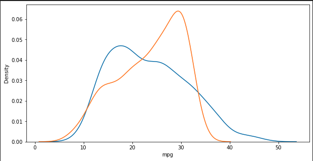
# 정답
list(y[0:10])

### 출력 결과
[18.0, 15.0, 18.0, 16.0, 17.0, 15.0, 14.0, 14.0, 14.0, 15.0]

# 예측값
y_hat[0:10]

### 출력 결과
array([19.54234168, 18.0769431 , 20.06957503, 20.09283533, 19.96878042,
       13.05271937, 12.95192476, 13.27756889, 12.40143111, 16.85965432])
2-2) 다중 회귀 분석
# train data 와 test data로 구분(7:3 비율)
from sklearn.model_selection import train_test_split
X_train, X_test, y_train, y_test = train_test_split(X, y, test_size=0.3, random_state=10)

print('훈련 데이터: ', X_train.shape)
print('검증 데이터: ', X_test.shape)

### 출력 결과
훈련 데이터:  (274, 1)
검증 데이터:  (118, 1)

'''
Step 5: 비선형회귀분석 모형 - sklearn 사용
'''

# sklearn 라이브러리에서 필요한 모듈 가져오기
from sklearn.linear_model import LinearRegression      #선형회귀분석
from sklearn.preprocessing import PolynomialFeatures   #다항식 변환

# 다항식 변환
poly = PolynomialFeatures(degree=2)               #2차항 적용
X_train_poly=poly.fit_transform(X_train)     #X_train 데이터를 2차항으로 변형

print('원 데이터: ', X_train.shape)
print('2차항 변환 데이터: ', X_train_poly.shape)

### 출력 결과
원 데이터:  (274, 1)
2차항 변환 데이터:  (274, 3)
X_train.head()
### 출력 결과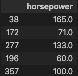
X_train_poly[:5]

### 출력 결과
array([[1.0000e+00, 1.6500e+02, 2.7225e+04],
       [1.0000e+00, 7.1000e+01, 5.0410e+03],
       [1.0000e+00, 1.3300e+02, 1.7689e+04],
       [1.0000e+00, 6.0000e+01, 3.6000e+03],
       [1.0000e+00, 1.0000e+02, 1.0000e+04]])
# train data를 가지고 모형 학습
pr = LinearRegression()
pr.fit(X_train_poly, y_train)
### 출력 결과
LinearRegression()
# 학습을 마친 모형에 test data를 적용하여 결정계수(R-제곱) 계산
X_test_poly = poly.fit_transform(X_test) #X_test 데이터를 2차항으로 변형
r_square = pr.score(X_test_poly,y_test)
print(r_square)
### 출력 결과
0.7066920352416861
# 회귀식의 기울기
print('기울기 a: ', pr.coef_)
### 출력 결과
기울기 a: [ 0. -0.44239775 0.00113262]
# 회귀식의 y절편
print('y절편 b', pr.intercept_)
### 출력 결과
y절편 b 55.99491066376761# train data의 산점도와 test data로 예측한 회귀선을 그래프로 출력
y_hat_test = pr.predict(X_test_poly)
fig = plt.figure(figsize=(10, 5))
ax = fig.add_subplot(1, 1, 1)
ax.plot(X_train.values, y_train, 'o', label='Train Data') # 데이터 분포
ax.plot(X_test.values, y_hat_test, 'r+', label='Predicted Value') # 모형이 학습한 회귀선
ax.legend(loc='best')
plt.xlabel('weight')
plt.ylabel('mpg')
plt.show()
plt.close()
### 출력 결과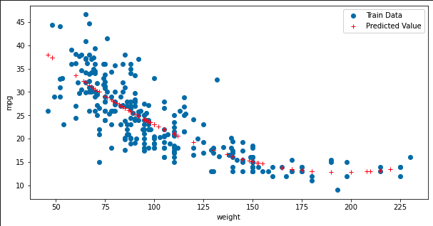
# 모형에 전체 X 데이터를 입력하여 예측한 값 y_hat을 실제 값 y와 비교
X_ploy = poly.fit_transform(X)
y_hat = pr.predict(X_ploy)

plt.figure(figsize=(10, 5))
ax1 = sns.distplot(y, hist=False, label="y")                 # 정답 : 파란색
ax2 = sns.distplot(y_hat, hist=False, label="y_hat", ax=ax1) # 예측 : 주황색
plt.show()
plt.close()

### 출력 결과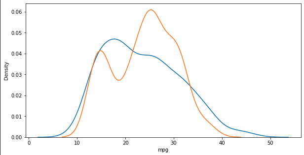
2-3) 다중 회귀 분석
'''
Step 4: 데이터셋 구분 - 훈련용(train data)/ 검증용(test data)
'''

# 속성(변수) 선택
X=ndf[['displacement','horsepower','weight']]  #독립 변수 X1, X2, X3
#X=ndf[['displacement','horsepower','weight', 'origin']]  #독립 변수 X1, X2, X3
y=ndf['mpg']     #종속 변수 Y

# train data 와 test data로 구분(7:3 비율)
from sklearn.model_selection import train_test_split
X_train, X_test, y_train, y_test = train_test_split(X, y, test_size=0.3, random_state=10)

print('훈련 데이터: ', X_train.shape)
print('검증 데이터: ', X_test.shape)

### 출력 결과
훈련 데이터:  (274, 3)
검증 데이터:  (118, 3)
'''
Step 5: 다중회귀분석 모형 - sklearn 사용
'''
# sklearn 라이브러리에서 선형회귀분석 모듈 가져오기
from sklearn.linear_model import LinearRegression
# 단순회귀분석 모형 객체 생성
lr = LinearRegression()
# train data를 가지고 모형 학습
lr.fit(X_train, y_train)
# 학습을 마친 모형에 test data를 적용하여 결정계수(R-제곱) 계산
r_square = lr.score(X_test, y_test)
print(r_square)
### 출력 결과
0.6993315144604407X_train.head()
### 출력 결과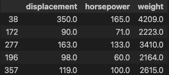
# 회귀식의 기울기
print('X 변수의 계수 a: ', lr.coef_)

### 출력 결과
X 변수의 계수 a:  [-0.00291301 -0.04314877 -0.00574424]

# 회귀식의 y절편
print('상수항 b', lr.intercept_)

### 출력 결과
상수항 b 45.83547601109956
# train data의 산점도와 test data로 예측한 회귀선을 그래프로 출력
y_hat = lr.predict(X_test)
plt.figure(figsize=(10, 5))
ax1 = sns.distplot(y_test, hist=False, label="y_test") # 정답 : 파란색
ax2 = sns.distplot(y_hat, hist=False, label="y_hat", ax=ax1) # 예측 : 주황색
plt.show()
plt.close()
### 출력 결과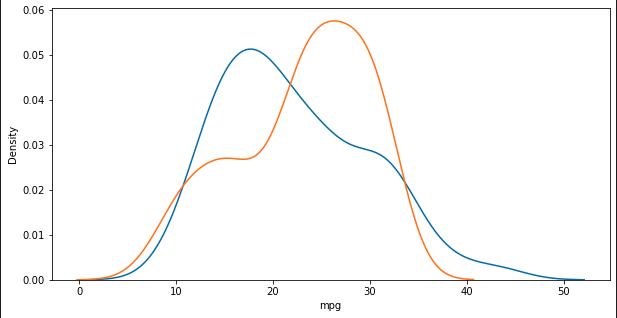
2-4) 실습
해당 실습에선 단순, 다항, 다중으로 모든 열들의 결과값을 출력해 볼 것이다.
단순 회귀
import pandas as pd
import numpy as np
import seaborn as sns
import matplotlib.pyplot as plt
from sklearn.linear_model import LinearRegression
from sklearn.model_selection import train_test_split

# CSV 파일을 데이터프레임으로 변환
df = pd.read_csv('data/auto-mpg.csv', header=None)

# 열 이름 지정
df.columns = ['mpg', 'cylinders', 'displacement', 'horsepower', 'weight',
              'acceleration', 'model year', 'origin', 'name']

# '?'을 np.nan으로 변경
df['horsepower'].replace('?', np.nan, inplace=True)

# 누락데이터 행을 삭제
df.dropna(subset=['horsepower'], axis=0, inplace=True)

# 문자열을 실수형으로 변환
df['horsepower'] = df['horsepower'].astype('float')

# 분석할 변수 목록
columns = ['mpg', 'cylinders', 'displacement', 'horsepower', 'weight']

# 결과를 저장할 리스트
results = []

# 각 변수에 대해 단순 회귀 분석 수행
for target_column in columns:
    for feature_column in columns:
        if feature_column != target_column:
            X = df[[feature_column]]  # 독립 변수
            y = df[target_column]     # 종속 변수

            # 데이터 분리 (7:3 비율)
            X_train, X_test, y_train, y_test = train_test_split(X, y, test_size=0.3, random_state=10)

            # 단순회귀분석 모형 객체 생성
            lr = LinearRegression()

            # train data를 가지고 모형 학습
            lr.fit(X_train, y_train)

            # 학습을 마친 모형에 test data를 적용하여 결정계수(R-제곱) 계산
            r_square = lr.score(X_test, y_test)

            # 회귀식의 기울기와 y절편
            coef = lr.coef_[0]
            intercept = lr.intercept_

            # 결과 저장
            results.append((feature_column, target_column, r_square, coef, intercept))

            # 모형에 전체 X 데이터를 입력하여 예측한 값 y_hat을 실제 값 y와 비교
            y_hat = lr.predict(X)

            # plt.figure(figsize=(10, 5))
            # ax1 = sns.distplot(y, hist=False, label="y")  # 정답 : 파란색
            # ax2 = sns.distplot(y_hat, hist=False, label="y_hat", ax=ax1)  # 예측값 : 주황색
            # plt.title(f'Simple Linear Regression\nFeature: {feature_column} -> Target: {target_column}')
            # plt.show()
            # plt.close()

# 결과 출력
for column in columns:
    column_results = [result for result in results if result[0] == column]
    highest_r2 = max(column_results, key=lambda x: x[2])
    lowest_r2 = min(column_results, key=lambda x: x[2])

    print(f'해당 열 {column}:')
    print(f'가장 높은 R스퀘어: {highest_r2[2]} (타겟: {highest_r2[1]})')
    print(f'가장 낮은 R스퀘어: {lowest_r2[2]} (타겟: {lowest_r2[1]})')
    print('\n')

print("-" * 50)
print("-" * 50)
print()

# 전체 결과 출력
for result in results:
    print(f'열: {result[0]} -> 타겟: {result[1]}')
    print(f'R스퀘어: {result[2]}')
    print(f'기울기 a: {result[3]}')
    print(f'y절편 b: {result[4]}')
    print('\n')

### 출력결과
해당 열 mpg:
가장 높은 R스퀘어: 0.6886221944358812 (타겟: weight)
가장 낮은 R스퀘어: 0.566940455699023 (타겟: cylinders)


해당 열 cylinders:
가장 높은 R스퀘어: 0.9057670998090408 (타겟: displacement)
가장 낮은 R스퀘어: 0.5444717222890907 (타겟: mpg)


해당 열 displacement:
가장 높은 R스퀘어: 0.9060967353543782 (타겟: cylinders)
가장 낮은 R스퀘어: 0.6460159729950312 (타겟: mpg)


해당 열 horsepower:
가장 높은 R스퀘어: 0.7433567953725483 (타겟: displacement)
가장 낮은 R스퀘어: 0.5956667983866819 (타겟: mpg)


해당 열 weight:
가장 높은 R스퀘어: 0.8766843149963266 (타겟: displacement)
가장 낮은 R스퀘어: 0.6822458558299322 (타겟: mpg)


--------------------------------------------------
--------------------------------------------------

열: cylinders -> 타겟: mpg
R스퀘어: 0.5444717222890907
기울기 a: -3.674913995676285
y절편 b: 43.85026412256791


열: displacement -> 타겟: mpg
R스퀘어: 0.6460159729950312
기울기 a: -0.06077765899422362
y절편 b: 35.51842669492941


열: horsepower -> 타겟: mpg
R스퀘어: 0.5956667983866819
기울기 a: -0.16090074717603686
y절편 b: 40.612861699281396


열: weight -> 타겟: mpg
R스퀘어: 0.6822458558299322
기울기 a: -0.007753431671236767
y절편 b: 46.7103662572801


열: mpg -> 타겟: cylinders
R스퀘어: 0.566940455699023
기울기 a: -0.16876613415078748
y절편 b: 9.45745296575539


열: displacement -> 타겟: cylinders
R스퀘어: 0.9060967353543782
기울기 a: 0.015436215372471498
y절편 b: 2.477093125725937


열: horsepower -> 타겟: cylinders
R스퀘어: 0.6294726870930445
기울기 a: 0.03840154612276222
y절편 b: 1.4384150346346183


열: weight -> 타겟: cylinders
R스퀘어: 0.8031340273852237
기울기 a: 0.0017933579377227124
y절편 b: 0.15085766553613755


열: mpg -> 타겟: displacement
R스퀘어: 0.6552648423886718
기울기 a: -10.574527387045816
y절편 b: 443.61935765460737


열: cylinders -> 타겟: displacement
R스퀘어: 0.9057670998090408
기울기 a: 58.481661810320496
y절편 b: -126.34593476830517


열: horsepower -> 타겟: displacement
R스퀘어: 0.7433567953725483
기울기 a: 2.494568727781829
y절편 b: -67.99399658093463


열: weight -> 타겟: displacement
R스퀘어: 0.8766843149963266
기울기 a: 0.11449881224283348
y절편 b: -145.76808397786553


열: mpg -> 타겟: horsepower
R스퀘어: 0.6106817872959865
기울기 a: -3.737731777763042
y절편 b: 193.08669082705995


열: cylinders -> 타겟: horsepower
R스퀘어: 0.6337145500928598
기울기 a: 19.424983551085624
y절편 b: -1.6265532474856457


열: displacement -> 타겟: horsepower
R스퀘어: 0.7491556207189045
기울기 a: 0.3330646549469245
y절편 b: 40.16672657200307


열: weight -> 타겟: horsepower
R스퀘어: 0.7461704764721846
기울기 a: 0.03883433750827423
y절편 b: -10.43519698610838


열: mpg -> 타겟: weight
R스퀘어: 0.6886221944358812
기울기 a: -89.20718328680178
y절편 b: 5072.164278897888


열: cylinders -> 타겟: weight
R스퀘어: 0.8002186084570136
기울기 a: 449.298242316007
y절편 b: 502.5197386972468


열: displacement -> 타겟: weight
R스퀘어: 0.8755273320320337
기울기 a: 7.571638069274184
y절편 b: 1494.349581029578


열: horsepower -> 타겟: weight
R스퀘어: 0.7409706707491546
기울기 a: 19.23409211059284
y절편 b: 943.6723788659292
다항 회귀
import pandas as pd
import numpy as np
import seaborn as sns
import matplotlib.pyplot as plt
from sklearn.linear_model import LinearRegression
from sklearn.model_selection import train_test_split
from sklearn.preprocessing import PolynomialFeatures   #다항식 변환

# CSV 파일을 데이터프레임으로 변환
df = pd.read_csv('data/auto-mpg.csv', header=None)

# 열 이름 지정
df.columns = ['mpg', 'cylinders', 'displacement', 'horsepower', 'weight',
              'acceleration', 'model year', 'origin', 'name']

# '?'을 np.nan으로 변경
df['horsepower'].replace('?', np.nan, inplace=True)

# 누락데이터 행을 삭제
df.dropna(subset=['horsepower'], axis=0, inplace=True)

# 문자열을 실수형으로 변환
df['horsepower'] = df['horsepower'].astype('float')

# 분석할 변수 목록
columns = ['mpg', 'cylinders', 'displacement', 'horsepower', 'weight']

# 결과를 저장할 리스트
results = []

# 각 변수에 대해 단순 회귀 분석 수행
for target_column in columns:
    for feature_column in columns:
        if feature_column != target_column:
            X = df[[feature_column]]  # 독립 변수
            y = df[target_column]     # 종속 변수

            # 데이터 분리 (7:3 비율)
            X_train, X_test, y_train, y_test = train_test_split(X, y, test_size=0.3, random_state=10)

            poly = PolynomialFeatures(degree=2)               #2차항 적용
            X_train_poly = poly.fit_transform(X_train)        #X_train 데이터를 2차항으로 변형

            # train data를 가지고 모형 학습
            pr = LinearRegression()
            pr.fit(X_train_poly, y_train)

            # 학습을 마친 모형에 test data를 적용하여 결정계수(R-제곱) 계산
            X_test_poly = poly.transform(X_test)       #X_test 데이터를 2차항으로 변형
            r_square = pr.score(X_test_poly, y_test)

            # 회귀식의 기울기와 y절편
            coef = pr.coef_
            intercept = pr.intercept_

            # 결과 저장
            results.append((feature_column, target_column, r_square, coef, intercept))

            # 모형에 전체 X 데이터를 입력하여 예측한 값 y_hat을 실제 값 y와 비교
            X_poly = poly.transform(X)
            y_hat = pr.predict(X_poly)

            # 그래프 표시
            # plt.figure(figsize=(10, 5))
            # ax1 = sns.distplot(y, hist=False, label="y")  # 정답 : 파란색
            # ax2 = sns.distplot(y_hat, hist=False, label="y_hat", ax=ax1)  # 예측값 : 주황색
            # plt.title(f'Simple Linear Regression\nFeature: {feature_column} -> Target: {target_column}')
            # plt.show()
            # plt.close()

# 결과 출력
for column in columns:
    column_results = [result for result in results if result[0] == column]
    highest_r2 = max(column_results, key=lambda x: x[2])
    lowest_r2 = min(column_results, key=lambda x: x[2])

    print(f'해당 열 {column}:')
    print(f'가장 높은 R스퀘어: {highest_r2[2]} (타겟: {highest_r2[1]})')
    print(f'가장 낮은 R스퀘어: {lowest_r2[2]} (타겟: {lowest_r2[1]})')
    print('\n')

print("-" * 50)
print("-" * 50)
print()

# 전체 결과 출력
for result in results:
    print(f'열: {result[0]} -> 타겟: {result[1]}')
    print(f'R스퀘어: {result[2]}')
    print(f'기울기 a: {result[3]}')
    print(f'y절편 b: {result[4]}')
    print('\n')

### 출력 결과
해당 열 mpg:
가장 높은 R스퀘어: 0.7920364159421698 (타겟: weight)
가장 낮은 R스퀘어: 0.674572034406353 (타겟: cylinders)


해당 열 cylinders:
가장 높은 R스퀘어: 0.9061821449011748 (타겟: displacement)
가장 낮은 R스퀘어: 0.5066072041897869 (타겟: mpg)


해당 열 displacement:
가장 높은 R스퀘어: 0.9189884891475524 (타겟: cylinders)
가장 낮은 R스퀘어: 0.6668796177413645 (타겟: mpg)


해당 열 horsepower:
가장 높은 R스퀘어: 0.7740599917610285 (타겟: weight)
가장 낮은 R스퀘어: 0.6562423690656733 (타겟: cylinders)


해당 열 weight:
가장 높은 R스퀘어: 0.8761942934183272 (타겟: displacement)
가장 낮은 R스퀘어: 0.7087009262975688 (타겟: mpg)


--------------------------------------------------
--------------------------------------------------

열: cylinders -> 타겟: mpg
R스퀘어: 0.5066072041897869
기울기 a: [  0.         -10.12043128   0.54448674]
y절편 b: 61.24457612494818


열: displacement -> 타겟: mpg
R스퀘어: 0.6668796177413645
기울기 a: [ 0.         -0.14784156  0.00018814]
y절편 b: 43.25466000393257


열: horsepower -> 타겟: mpg
R스퀘어: 0.7066920352416861
기울기 a: [ 0.         -0.44239775  0.00113262]
y절편 b: 55.99491066376761


열: weight -> 타겟: mpg
R스퀘어: 0.7087009262975688
기울기 a: [ 0.00000000e+00 -1.85768289e-02  1.70491223e-06]
y절편 b: 62.580712215731424


열: mpg -> 타겟: cylinders
R스퀘어: 0.674572034406353
기울기 a: [ 0.         -0.64440084  0.0093112 ]
y절편 b: 14.933238968111713


열: displacement -> 타겟: cylinders
R스퀘어: 0.9189884891475524
기울기 a: [ 0.00000000e+00  2.48658986e-02 -2.03769574e-05]
y절편 b: 1.63920019968816


열: horsepower -> 타겟: cylinders
R스퀘어: 0.6562423690656733
기울기 a: [ 0.          0.07447919 -0.00014516]
y절편 b: -0.533002367697363


열: weight -> 타겟: cylinders
R스퀘어: 0.80273403997759
기울기 a: [0.00000000e+00 1.61301462e-03 2.84078571e-08]
y절편 b: 0.4152950438305325


열: mpg -> 타겟: displacement
R스퀘어: 0.7590811324175315
기울기 a: [  0.         -39.13304478   0.5590719 ]
y절편 b: 772.4017756557286


열: cylinders -> 타겟: displacement
R스퀘어: 0.9061821449011748
기울기 a: [ 0.         21.99903765  3.08187914]
y절편 b: -27.891440031676694


열: horsepower -> 타겟: displacement
R스퀘어: 0.7531677565938584
기울기 a: [ 0.00000000e+00  3.12944044e+00 -2.55444002e-03]
y절편 b: -102.68576109376286


열: weight -> 타겟: displacement
R스퀘어: 0.8761942934183272
기울기 a: [0.00000000e+00 8.21567563e-02 5.09455264e-06]
y절편 b: -98.34493137726255


열: mpg -> 타겟: horsepower
R스퀘어: 0.722435535041228
기울기 a: [  0.         -13.10573591   0.18339145]
y절편 b: 300.9366540836461


열: cylinders -> 타겟: horsepower
R스퀘어: 0.7113788145124411
기울기 a: [  0.         -22.0942294    3.50734628]
y절편 b: 110.42002307887289


열: displacement -> 타겟: horsepower
R스퀘어: 0.787292468898066
기울기 a: [0.         0.07895962 0.00054911]
y절편 b: 62.74572575820881


열: weight -> 타겟: horsepower
R스퀘어: 0.7624851614525514
기울기 a: [0.00000000e+00 1.35565143e-02 3.98178772e-06]
y절편 b: 26.629672098883432


열: mpg -> 타겟: weight
R스퀘어: 0.7920364159421698
기울기 a: [   0.         -292.59106096    3.98151656]
y절편 b: 7413.6388783111615


열: cylinders -> 타겟: weight
R스퀘어: 0.7969890010515097
기울기 a: [  0.         538.53096989  -7.5379578 ]
y절편 b: 261.7102215971072


열: displacement -> 타겟: weight
R스퀘어: 0.8708653281894765
기울기 a: [ 0.00000000e+00  1.32675266e+01 -1.23084598e-02]
y절편 b: 988.230279728109


열: horsepower -> 타겟: weight
R스퀘어: 0.7740599917610285
기울기 a: [ 0.         40.32233068 -0.08484965]
y절편 b: -208.66783988100497
다중 회귀
import pandas as pd
import numpy as np
import seaborn as sns
import matplotlib.pyplot as plt
from sklearn.linear_model import LinearRegression
from sklearn.model_selection import train_test_split
from sklearn.preprocessing import PolynomialFeatures   # 다항식 변환

# CSV 파일을 데이터프레임으로 변환
df = pd.read_csv('data/auto-mpg.csv', header=None)

# 열 이름 지정
df.columns = ['mpg', 'cylinders', 'displacement', 'horsepower', 'weight',
              'acceleration', 'model year', 'origin', 'name']

# '?'을 np.nan으로 변경
df['horsepower'].replace('?', np.nan, inplace=True)

# 누락데이터 행을 삭제
df.dropna(subset=['horsepower'], axis=0, inplace=True)

# 문자열을 실수형으로 변환
df['horsepower'] = df['horsepower'].astype('float')

# 분석할 변수 목록
columns = ['mpg', 'cylinders', 'displacement', 'horsepower', 'weight']

# 결과를 저장할 리스트
results = []

# 각 변수에 대해 단순 회귀 분석 수행
for target_column in columns:
    for feature_column in columns:
        if feature_column != target_column:
            X = df[[feature_column]]  # 독립 변수
            y = df[target_column]     # 종속 변수

            # 데이터 분리 (7:3 비율)
            X_train, X_test, y_train, y_test = train_test_split(X, y, test_size=0.3, random_state=10)

            for degree in [1, 2]:  # 1차와 2차 회귀를 수행
                poly = PolynomialFeatures(degree=degree)  # 다항식 차수 설정
                X_train_poly = poly.fit_transform(X_train)  # X_train 데이터를 변형

                # train data를 가지고 모형 학습
                pr = LinearRegression()
                pr.fit(X_train_poly, y_train)

                # 학습을 마친 모형에 test data를 적용하여 결정계수(R-제곱) 계산
                X_test_poly = poly.transform(X_test)  # X_test 데이터를 변형
                r_square = pr.score(X_test_poly, y_test)

                # 회귀식의 기울기와 y절편
                coef = pr.coef_
                intercept = pr.intercept_

                # 결과 저장
                results.append((feature_column, target_column, degree, r_square, coef, intercept))

                # 모형에 전체 X 데이터를 입력하여 예측한 값 y_hat을 실제 값 y와 비교
                X_poly = poly.transform(X)
                y_hat = pr.predict(X_poly)

                # 그래프 표시
                # plt.figure(figsize=(10, 5))
                # ax1 = sns.distplot(y, hist=False, label="y")  # 정답 : 파란색
                # ax2 = sns.distplot(y_hat, hist=False, label="y_hat", ax=ax1)  # 예측값 : 주황색
                # plt.title(f'Polynomial Regression (degree={degree})\nFeature: {feature_column} -> Target: {target_column}')
                # plt.show()
                # plt.close()

# 결과 출력
for column in columns:
    column_results = [result for result in results if result[0] == column]
    highest_r2 = max(column_results, key=lambda x: x[3])
    lowest_r2 = min(column_results, key=lambda x: x[3])

    print(f'해당 열 {column}:')
    print(f'가장 높은 R스퀘어: {highest_r2[3]} (타겟: {highest_r2[1]}, 차수: {highest_r2[2]})')
    print(f'가장 낮은 R스퀘어: {lowest_r2[3]} (타겟: {lowest_r2[1]}, 차수: {lowest_r2[2]})')
    print('\n')

print("-" * 50)
print("-" * 50)
print()

# 전체 결과 출력
for result in results:
    print(f'열: {result[0]} -> 타겟: {result[1]} (차수: {result[2]})')
    print(f'R스퀘어: {result[3]}')
    print(f'기울기 a: {result[4]}')
    print(f'y절편 b: {result[5]}')
    print('\n')

### 출력 결과
해당 열 mpg:
가장 높은 R스퀘어: 0.7920364159421698 (타겟: weight, 차수: 2)
가장 낮은 R스퀘어: 0.5669404556990228 (타겟: cylinders, 차수: 1)


해당 열 cylinders:
가장 높은 R스퀘어: 0.9061821449011748 (타겟: displacement, 차수: 2)
가장 낮은 R스퀘어: 0.5066072041897869 (타겟: mpg, 차수: 2)


해당 열 displacement:
가장 높은 R스퀘어: 0.9189884891475524 (타겟: cylinders, 차수: 2)
가장 낮은 R스퀘어: 0.6460159729950312 (타겟: mpg, 차수: 1)


해당 열 horsepower:
가장 높은 R스퀘어: 0.7740599917610285 (타겟: weight, 차수: 2)
가장 낮은 R스퀘어: 0.5956667983866821 (타겟: mpg, 차수: 1)


해당 열 weight:
가장 높은 R스퀘어: 0.8766843149963266 (타겟: displacement, 차수: 1)
가장 낮은 R스퀘어: 0.6822458558299325 (타겟: mpg, 차수: 1)


--------------------------------------------------
--------------------------------------------------

열: cylinders -> 타겟: mpg (차수: 1)
R스퀘어: 0.5444717222890907
기울기 a: [ 0.       -3.674914]
y절편 b: 43.85026412256791


열: cylinders -> 타겟: mpg (차수: 2)
R스퀘어: 0.5066072041897869
기울기 a: [  0.         -10.12043128   0.54448674]
y절편 b: 61.24457612494818


열: displacement -> 타겟: mpg (차수: 1)
R스퀘어: 0.6460159729950312
기울기 a: [ 0.         -0.06077766]
y절편 b: 35.51842669492942


열: displacement -> 타겟: mpg (차수: 2)
R스퀘어: 0.6668796177413645
기울기 a: [ 0.         -0.14784156  0.00018814]
y절편 b: 43.25466000393257


열: horsepower -> 타겟: mpg (차수: 1)
R스퀘어: 0.5956667983866821
기울기 a: [ 0.         -0.16090075]
y절편 b: 40.61286169928138


열: horsepower -> 타겟: mpg (차수: 2)
R스퀘어: 0.7066920352416861
기울기 a: [ 0.         -0.44239775  0.00113262]
y절편 b: 55.99491066376761


열: weight -> 타겟: mpg (차수: 1)
R스퀘어: 0.6822458558299325
기울기 a: [ 0.         -0.00775343]
y절편 b: 46.710366257280086


열: weight -> 타겟: mpg (차수: 2)
R스퀘어: 0.7087009262975688
기울기 a: [ 0.00000000e+00 -1.85768289e-02  1.70491223e-06]
y절편 b: 62.580712215731424


열: mpg -> 타겟: cylinders (차수: 1)
R스퀘어: 0.5669404556990228
기울기 a: [ 0.         -0.16876613]
y절편 b: 9.457452965755394


열: mpg -> 타겟: cylinders (차수: 2)
R스퀘어: 0.674572034406353
기울기 a: [ 0.         -0.64440084  0.0093112 ]
y절편 b: 14.933238968111713


열: displacement -> 타겟: cylinders (차수: 1)
R스퀘어: 0.9060967353543782
기울기 a: [0.         0.01543622]
y절편 b: 2.4770931257259345


열: displacement -> 타겟: cylinders (차수: 2)
R스퀘어: 0.9189884891475524
기울기 a: [ 0.00000000e+00  2.48658986e-02 -2.03769574e-05]
y절편 b: 1.63920019968816


열: horsepower -> 타겟: cylinders (차수: 1)
R스퀘어: 0.6294726870930445
기울기 a: [0.         0.03840155]
y절편 b: 1.4384150346346192


열: horsepower -> 타겟: cylinders (차수: 2)
R스퀘어: 0.6562423690656733
기울기 a: [ 0.          0.07447919 -0.00014516]
y절편 b: -0.533002367697363


열: weight -> 타겟: cylinders (차수: 1)
R스퀘어: 0.8031340273852237
기울기 a: [0.         0.00179336]
y절편 b: 0.15085766553613844


열: weight -> 타겟: cylinders (차수: 2)
R스퀘어: 0.80273403997759
기울기 a: [0.00000000e+00 1.61301462e-03 2.84078571e-08]
y절편 b: 0.4152950438305325


열: mpg -> 타겟: displacement (차수: 1)
R스퀘어: 0.6552648423886718
기울기 a: [  0.         -10.57452739]
y절편 b: 443.6193576546076


열: mpg -> 타겟: displacement (차수: 2)
R스퀘어: 0.7590811324175315
기울기 a: [  0.         -39.13304478   0.5590719 ]
y절편 b: 772.4017756557286


열: cylinders -> 타겟: displacement (차수: 1)
R스퀘어: 0.9057670998090408
기울기 a: [ 0.         58.48166181]
y절편 b: -126.34593476830534


열: cylinders -> 타겟: displacement (차수: 2)
R스퀘어: 0.9061821449011748
기울기 a: [ 0.         21.99903765  3.08187914]
y절편 b: -27.891440031676694


열: horsepower -> 타겟: displacement (차수: 1)
R스퀘어: 0.7433567953725484
기울기 a: [0.         2.49456873]
y절편 b: -67.99399658093441


열: horsepower -> 타겟: displacement (차수: 2)
R스퀘어: 0.7531677565938584
기울기 a: [ 0.00000000e+00  3.12944044e+00 -2.55444002e-03]
y절편 b: -102.68576109376286


열: weight -> 타겟: displacement (차수: 1)
R스퀘어: 0.8766843149963266
기울기 a: [0.         0.11449881]
y절편 b: -145.76808397786547


열: weight -> 타겟: displacement (차수: 2)
R스퀘어: 0.8761942934183272
기울기 a: [0.00000000e+00 8.21567563e-02 5.09455264e-06]
y절편 b: -98.34493137726255


열: mpg -> 타겟: horsepower (차수: 1)
R스퀘어: 0.6106817872959867
기울기 a: [ 0.         -3.73773178]
y절편 b: 193.08669082706


열: mpg -> 타겟: horsepower (차수: 2)
R스퀘어: 0.722435535041228
기울기 a: [  0.         -13.10573591   0.18339145]
y절편 b: 300.9366540836461


열: cylinders -> 타겟: horsepower (차수: 1)
R스퀘어: 0.6337145500928598
기울기 a: [ 0.         19.42498355]
y절편 b: -1.6265532474856457


열: cylinders -> 타겟: horsepower (차수: 2)
R스퀘어: 0.7113788145124411
기울기 a: [  0.         -22.0942294    3.50734628]
y절편 b: 110.42002307887289


열: displacement -> 타겟: horsepower (차수: 1)
R스퀘어: 0.7491556207189045
기울기 a: [0.         0.33306465]
y절편 b: 40.16672657200307


열: displacement -> 타겟: horsepower (차수: 2)
R스퀘어: 0.787292468898066
기울기 a: [0.         0.07895962 0.00054911]
y절편 b: 62.74572575820881


열: weight -> 타겟: horsepower (차수: 1)
R스퀘어: 0.7461704764721845
기울기 a: [0.         0.03883434]
y절편 b: -10.435196986108323


열: weight -> 타겟: horsepower (차수: 2)
R스퀘어: 0.7624851614525514
기울기 a: [0.00000000e+00 1.35565143e-02 3.98178772e-06]
y절편 b: 26.629672098883432


열: mpg -> 타겟: weight (차수: 1)
R스퀘어: 0.6886221944358812
기울기 a: [  0.         -89.20718329]
y절편 b: 5072.16427889789


열: mpg -> 타겟: weight (차수: 2)
R스퀘어: 0.7920364159421698
기울기 a: [   0.         -292.59106096    3.98151656]
y절편 b: 7413.6388783111615


열: cylinders -> 타겟: weight (차수: 1)
R스퀘어: 0.8002186084570138
기울기 a: [  0.         449.29824232]
y절편 b: 502.5197386972459


열: cylinders -> 타겟: weight (차수: 2)
R스퀘어: 0.7969890010515097
기울기 a: [  0.         538.53096989  -7.5379578 ]
y절편 b: 261.7102215971072


열: displacement -> 타겟: weight (차수: 1)
R스퀘어: 0.8755273320320338
기울기 a: [0.         7.57163807]
y절편 b: 1494.3495810295772


열: displacement -> 타겟: weight (차수: 2)
R스퀘어: 0.8708653281894765
기울기 a: [ 0.00000000e+00  1.32675266e+01 -1.23084598e-02]
y절편 b: 988.230279728109


열: horsepower -> 타겟: weight (차수: 1)
R스퀘어: 0.7409706707491546
기울기 a: [ 0.         19.23409211]
y절편 b: 943.672378865931


열: horsepower -> 타겟: weight (차수: 2)
R스퀘어: 0.7740599917610285
기울기 a: [ 0.         40.32233068 -0.08484965]
y절편 b: -208.66783988100497
결론
상관이 높다 = 잘 맞춘다
상관이 적다 = 못 맞춘다
1. 연비
- 연비와 가장 상관이 높은건 무게이다.
- 실린더 수는 상관이 적다
2. 실린더
- 실린더와 가장 상관이 높은건 배기량이다
- 연비와는 상관이 적다
3. 배기량
- 배기량과 가장 상관이 높은건 실런더이다
- 연비와는 상관이 적다
4. 마력
- 마력과 가장 상관이 높은건 배기량이다
- 연비와는 상관이 적다
5. 무게
- 무게와 가장 상관이 높은건 배기량이다
- 연비와는 상관이 적다
3. 분류 분석
분류 분석이란?
분류(Classification)는 머신러닝에서 데이터 포인트를 미리 정의된 클래스 레이블 중 하나로 분류하는 작업.
분류 분석은 주로 이산형 데이터(정해진 범주의 데이터)를 처리하는 데 사용되며, 다양한 알고리즘과 기술을 사용하여 구현.
주요 개념
- 훈련 데이터(Training Data): 모델을 학습시키기 위해 사용하는 데이터로, 각 데이터 포인트는 입력(features)과 정답(label, class)으로 구성.
- 테스트 데이터(Test Data): 학습된 모델의 성능을 평가하기 위해 사용하는 데이터로, 모델이 예측한 결과와 실제 라벨을 비교하여 정확도를 측정.
- 특징(Features): 각 데이터 포인트를 설명하는 속성들.
예를 들어, 이메일 분류에서는 이메일의 단어 빈도, 길이 등이 특징이 될 수 있음.
- 라벨(Labels): 각 데이터 포인트가 속하는 클래스.
예를 들어, 스팸 이메일 분류에서는 '스팸' 또는 '정상'이 라벨이 됨.
- 모델(Model): 학습 과정을 통해 생성된 함수로, 새로운 데이터 포인트를 입력받아 클래스 레이블을 예측.
- 정확도(Accuracy): 모델이 올바르게 예측한 데이터 포인트의 비율.
하지만 데이터의 불균형이 있을 경우, 정밀도(Precision), 재현율(Recall), F1 점수 등 다른 평가 지표도 사용됨.
주요 분류 알고리즘
1. K-최근접 이웃(K-Nearest Neighbors, KNN):
- 새로운 데이터 포인트를 예측할 때, 가장 가까운 K개의 이웃 데이터를 기준으로 다수결 원칙에 따라 분류.
- 단순하고 이해하기 쉽지만, 계산 비용이 많이 들 수 있음.
2. 서포트 벡터 머신(SVM, Support Vector Machine):
- 클래스 간의 경계를 최대한 넓게 만드는 초평면(hyperplane)을 찾음.
- 고차원 공간에서도 효과적으로 작동하며, 커널 트릭을 통해 비선형 분류도 수행할 수 있음.
3. 결정 트리(Decision Tree):
- 데이터의 특징들을 기준으로 트리 구조를 생성하여 분류.
- 각 노드는 특징을 기준으로 데이터를 분할하고, 잎(leaf) 노드는 최종 클래스 레이블을 나타냄.
분류 분석의 적용 사례
- 이메일 스팸 필터링: 이메일을 '스팸' 또는 '정상'으로 분류.
- 이미지 인식: 이미지 데이터를 '고양이', '개', '자동차' 등으로 분류.
- 의료 진단: 환자의 진단 데이터를 기반으로 특정 질병 여부를 분류.
- 신용 리스크 평가: 대출 신청자의 데이터를 바탕으로 '신용 등급' 분류.
- 추천 시스템: 사용자의 과거 행동을 기반으로 '관심 있을 만한 제품' 분류.
분류 분석의 과정
- 데이터 수집 및 준비: 데이터를 수집하고, 누락된 값 처리, 정규화 등 전처리 작업 수행.
- 특징 선택 및 추출: 모델에 가장 중요한 특징들을 선택하고, 필요 시 새로운 특징을 생성.
- 모델 학습: 훈련 데이터를 사용하여 분류 모델 학습.
- 모델 평가: 테스트 데이터를 사용하여 모델의 성능 평가.
- 하이퍼파라미터 튜닝: 모델의 성능을 최적화하기 위해 하이퍼파라미터 조정.
- 배포 및 유지 관리: 최적화된 모델을 실제 환경에 배포하고, 성능을 모니터링 및 유지 관리.
3-1) KNN 분류
### 기본 라이브러리 불러오기
import pandas as pd
import seaborn as sns

'''
[Step 1] 데이터 준비 - Seaborn에서 제공하는 titanic 데이터셋 가져오기
'''
# load_dataset 함수를 사용하여 데이터프레임으로 변환
df = sns.load_dataset('titanic')

# 데이터 살펴보기
df.head()

### 출력 결과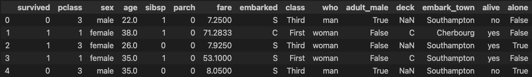
'''
[Step 2] 데이터 탐색
'''
# 데이터 자료형 확인
df.info()

### 출력 결과
<class 'pandas.core.frame.DataFrame'>
RangeIndex: 891 entries, 0 to 890
Data columns (total 15 columns):
 #   Column       Non-Null Count  Dtype
---  ------       --------------  -----
 0   survived     891 non-null    int64
 1   pclass       891 non-null    int64
 2   sex          891 non-null    object
 3   age          714 non-null    float64
 4   sibsp        891 non-null    int64
 5   parch        891 non-null    int64
 6   fare         891 non-null    float64
 7   embarked     889 non-null    object
 8   class        891 non-null    category
 9   who          891 non-null    object
 10  adult_male   891 non-null    bool
 11  deck         203 non-null    category
 12  embark_town  889 non-null    object
 13  alive        891 non-null    object
 14  alone        891 non-null    bool
dtypes: bool(2), category(2), float64(2), int64(4), object(5)
memory usage: 80.7+ KB
# NaN값이 많은 deck 열을 삭제, embarked와 내용이 겹치는 embark_town 열을 삭제
rdf = df.drop(['deck', 'embark_town'], axis=1)
rdf.columns
### 출력 결과
Index(['survived', 'pclass', 'sex', 'age', 'sibsp', 'parch', 'fare',
'embarked', 'class', 'who', 'adult_male', 'alive', 'alone'],
dtype='object')
# age 열에 나이 데이터가 없는 모든 행을 삭제 - age 열(891개 중 177개의 NaN 값)
rdf = rdf.dropna(subset=['age'], how='any', axis=0)
len(rdf)
### 출력 결과
714
rdf['embarked'].value_counts()
### 출력 결과
S 554
C 130
Q 28
Name: embarked, dtype: int64
# embarked 열의 NaN값을 승선도시 중에서 가장 많이 출현한 값으로 치환하기
most_freq = rdf['embarked'].value_counts(dropna=True).idxmax()
most_freq
### 출력 결과
'S'rdf.describe(include='all')
### 출력 결과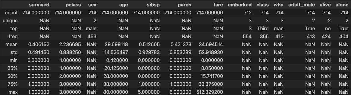
rdf['embarked'].fillna(most_freq, inplace=True)

'''
[Step 3] 분석에 사용할 속성을 선택
'''
# 분석에 활용할 열(속성)을 선택
ndf = rdf[['survived', 'pclass', 'sex', 'age', 'sibsp', 'parch', 'embarked']]
ndf.head()

### 출력 결과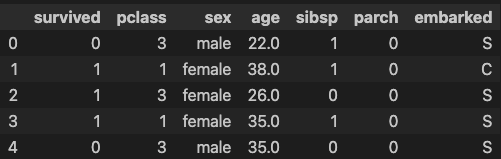
# 원핫인코딩 - 범주형 데이터를 모형이 인식할 수 있도록 숫자형으로 변환
onehot_sex = pd.get_dummies(ndf['sex'])
ndf = pd.concat([ndf, onehot_sex], axis=1)
ndf

### 출력 결과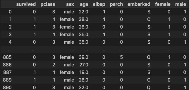
onehot_embarked = pd.get_dummies(ndf['embarked'], prefix='town')
ndf = pd.concat([ndf, onehot_embarked], axis=1)
ndf

### 출력 결과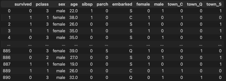
ndf.drop(['sex', 'embarked'], axis=1, inplace=True)
ndf.head()

### 출력 결과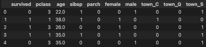
'''
[Step 4] 데이터셋 구분 - 훈련용(train data)/ 검증용(test data)
'''
# 속성(변수) 선택
X=ndf[['pclass', 'age', 'sibsp', 'parch', 'female', 'male',
       'town_C', 'town_Q', 'town_S']]  #독립 변수 X
y=ndf['survived']                      #종속 변수 Y

X.describe()

### 출력 결과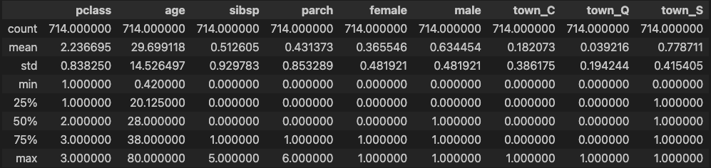
# 설명 변수 데이터를 정규화(normalization)
from sklearn import preprocessing
X = preprocessing.StandardScaler().fit(X).transform(X)
X

### 출력 결과
array([[ 0.91123237, -0.53037664,  0.52457013, ..., -0.47180795,
        -0.20203051,  0.53307848],
       [-1.47636364,  0.57183099,  0.52457013, ...,  2.11950647,
        -0.20203051, -1.87589641],
       [ 0.91123237, -0.25482473, -0.55170307, ..., -0.47180795,
        -0.20203051,  0.53307848],
       ...,
       [-1.47636364, -0.73704057, -0.55170307, ..., -0.47180795,
        -0.20203051,  0.53307848],
       [-1.47636364, -0.25482473, -0.55170307, ...,  2.11950647,
        -0.20203051, -1.87589641],
       [ 0.91123237,  0.15850313, -0.55170307, ..., -0.47180795,
         4.94974747, -1.87589641]])

# train data 와 test data로 구분(7:3 비율)
from sklearn.model_selection import train_test_split
X_train, X_test, y_train, y_test = train_test_split(X, y, test_size=0.3, random_state=10)

print('train data 개수: ', X_train.shape)
print('test data 개수: ', X_test.shape)

### 출력 결과
train data 개수:  (499, 9)
test data 개수:  (215, 9)
'''
[Step 5] KNN 분류 모형 - sklearn 사용
'''
# sklearn 라이브러리에서 KNN 분류 모형 가져오기
from sklearn.neighbors import KNeighborsClassifier
# 모형 객체 생성 (k=5로 설정)
knn = KNeighborsClassifier(n_neighbors=5)
# train data를 가지고 모형 학습
knn.fit(X_train, y_train)
### 출력 결과
KNeighborsClassifier()
# test data를 가지고 y_hat을 예측 (분류)
y_hat = knn.predict(X_test)
print(y_hat) # 예측값
print("--------------------------------------------------------------------")
print(y_test.values) # 정답
### 출력 결과
[0 0 1 0 0 1 1 1 0 0 1 1 0 0 0 1 0 0 1 1 1 0 0 1 0 0 1 0 0 0 0 0 0 1 0 0 1
0 1 1 0 1 1 0 0 0 0 0 1 1 1 0 1 1 1 1 0 0 0 0 1 0 1 0 0 1 1 0 0 0 0 1 1 0
0 0 0 0 0 0 1 0 0 0 0 0 0 0 1 1 1 0 0 1 1 0 0 0 0 0 1 0 1 0 0 0 0 1 1 0 0
0 1 0 0 0 1 0 1 1 1 0 0 0 0 0 0 1 0 0 0 0 1 0 1 0 0 0 1 0 1 0 1 0 0 0 1 1
0 1 0 1 0 0 0 0 1 0 0 1 0 0 0 1 0 1 0 1 0 1 0 0 0 1 1 0 1 1 0 1 0 1 0 1 1
0 1 0 0 0 1 0 0 0 1 1 0 1 1 0 0 1 0 0 0 0 1 1 0 0 0 0 0 0 1]
--------------------------------------------------------------------
[0 0 1 0 0 1 1 1 0 0 1 0 0 0 0 1 0 0 0 1 1 0 0 1 1 1 1 0 1 0 0 0 1 1 0 0 1
0 1 1 0 1 0 0 0 0 0 0 1 1 1 0 1 1 1 1 0 0 0 0 1 0 1 0 0 1 1 1 0 0 0 1 0 1
0 1 0 0 0 0 1 0 1 1 0 0 0 1 1 1 1 0 0 1 1 0 0 0 0 0 1 0 1 0 0 0 0 0 0 0 0
0 1 1 0 0 1 1 1 1 1 1 0 0 0 0 0 1 0 0 0 0 0 0 0 0 1 0 1 1 1 0 0 0 0 0 1 0
1 1 1 1 0 0 1 0 1 0 0 1 0 0 1 1 0 1 0 1 0 1 1 0 0 1 1 0 1 1 0 1 1 1 0 1 1
0 0 0 0 0 1 0 0 0 1 1 0 1 1 0 0 0 1 0 0 0 1 0 0 1 0 0 0 1 0]num = 0
for i,v in zip(y_hat, y_test.values):
if i == v:
num += 1
print(f"{num}개 정답")
### 출력 결과
177개 정답
print(f"정답률 : {num / len(y_hat):.2f}")
### 출력 결과
정답률 : 0.82
# 모형 성능 평가 - Confusion Matrix 계산
from sklearn import metrics
knn_matrix = metrics.confusion_matrix(y_test, y_hat)
print(knn_matrix)
### 출력 결과
[[111 14]
[ 24 66]]
# 모형 성능 평가 - 평가지표 계산
knn_report = metrics.classification_report(y_test, y_hat)
print(knn_report)
### 출력 결과
precision recall f1-score support
0 0.82 0.89 0.85 125
1 0.82 0.73 0.78 90
accuracy 0.82 215
macro avg 0.82 0.81 0.82 215
weighted avg 0.82 0.82 0.82 2153-2) SVM 분류
'''
[Step 5] SVM 분류 모형 - sklearn 사용
'''
# sklearn 라이브러리에서 SVM 분류 모형 가져오기
from sklearn import svm

# 모형 객체 생성 (kernel='rbf' 적용)
svm_model = svm.SVC(kernel='rbf')

# train data를 가지고 모형 학습
svm_model.fit(X_train, y_train)

### 출력 결과
SVC()

# test data를 가지고 y_hat을 예측 (분류)
y_hat = svm_model.predict(X_test)

# 예측값
print(y_hat[0:20])
# 정답
print(y_test.values[0:20])

### 출력 결과
[0 0 1 0 0 0 1 0 0 0 1 1 0 0 0 1 0 0 0 0]
[0 0 1 0 0 1 1 1 0 0 1 0 0 0 0 1 0 0 0 1]

# 모형 성능 평가 - Confusion Matrix 계산
from sklearn import metrics
svm_matrix = metrics.confusion_matrix(y_test, y_hat)
svm_matrix

### 출력 결과
array([[120,   5],
       [ 35,  55]])

# 모형 성능 평가 - 평가지표 계산
svm_report = metrics.classification_report(y_test, y_hat)
print(svm_report)

### 출력 결과
              precision    recall  f1-score   support

           0       0.77      0.96      0.86       125
           1       0.92      0.61      0.73        90

    accuracy                           0.81       215
   macro avg       0.85      0.79      0.80       215
weighted avg       0.83      0.81      0.81       215
3-3) 의사 결정 나무 (Decision Tree)
# -*- coding: utf-8 -*-
### 기본 라이브러리 불러오기
import pandas as pd
import numpy as np

'''
[Step 1] 데이터 준비/ 기본 설정
'''
# Breast Cancer 데이터셋 가져오기 (출처: UCI ML Repository)
uci_path = 'https://archive.ics.uci.edu/ml/machine-learning-databases/\
breast-cancer-wisconsin/breast-cancer-wisconsin.data'
df = pd.read_csv(uci_path, header=None)
df

### 출력 결과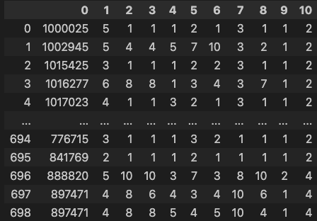
# 열 이름 지정
df.columns = ['id','clump','cell_size','cell_shape', 'adhesion','epithlial',
              'bare_nuclei','chromatin','normal_nucleoli', 'mitoses', 'class']
#  IPython 디스플레이 설정 - 출력할 열의 개수 한도 늘리기
pd.set_option('display.max_columns', 15)
df

### 출력 결과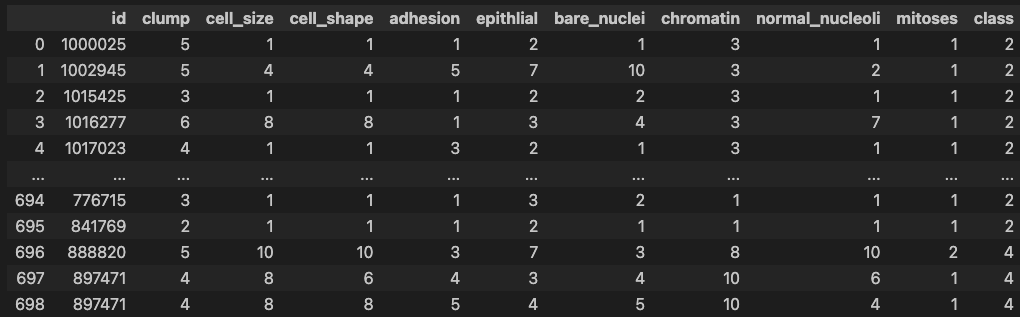
'''
[Step 2] 데이터 탐색
'''
# 데이터 살펴보기
df.head()

### 출력 결과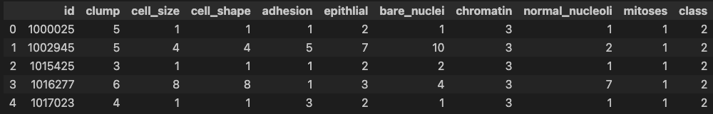
df.info()

### 출력 결과
<class 'pandas.core.frame.DataFrame'>
RangeIndex: 699 entries, 0 to 698
Data columns (total 11 columns):
 #   Column           Non-Null Count  Dtype
---  ------           --------------  -----
 0   id               699 non-null    int64
 1   clump            699 non-null    int64
 2   cell_size        699 non-null    int64
 3   cell_shape       699 non-null    int64
 4   adhesion         699 non-null    int64
 5   epithlial        699 non-null    int64
 6   bare_nuclei      699 non-null    object
 7   chromatin        699 non-null    int64
 8   normal_nucleoli  699 non-null    int64
 9   mitoses          699 non-null    int64
 10  class            699 non-null    int64
dtypes: int64(10), object(1)
memory usage: 60.2+ KB
# 데이터 통계 요약정보 확인
df.describe()
### 출력 결과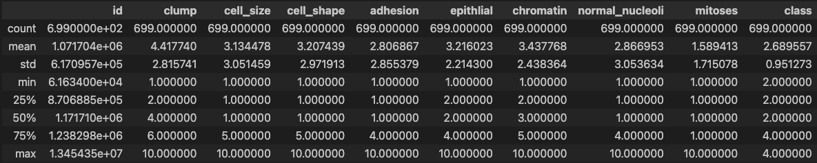
# bare_nuclei 열의 자료형 변경 (문자열 ->숫자)
df['bare_nuclei'].unique()                         # bare_nuclei 열의 고유값 확인

### 출력 결과
array(['1', '10', '2', '4', '3', '9', '7', '?', '5', '8', '6'],
      dtype=object)

df['bare_nuclei'].replace('?', np.nan, inplace=True)      # '?'을 np.nan으로 변경
df.dropna(subset=['bare_nuclei'], axis=0, inplace=True)   # 누락데이터 행을 삭제
df['bare_nuclei'] = df['bare_nuclei'].astype('int')       # 문자열을 정수형으로 변환

df.describe()                                      # 데이터 통계 요약정보 확인

### 출력 결과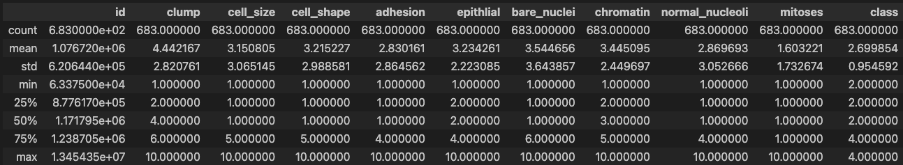
df['class'].unique()

### 출력 결과
array([2, 4])
'''
[Step 3] 데이터셋 구분 - 훈련용(train data)/ 검증용(test data)
'''
# 속성(변수) 선택
X=df[['clump','cell_size','cell_shape', 'adhesion','epithlial',
'bare_nuclei','chromatin','normal_nucleoli', 'mitoses']] #설명 변수 X
y=df['class'] #예측 변수 Y
y.unique()
### 출력 결과
array([2, 4])# 설명 변수 데이터를 정규화
from sklearn import preprocessing
X = preprocessing.StandardScaler().fit(X).transform(X)
# train data 와 test data로 구분(7:3 비율)
from sklearn.model_selection import train_test_split
X_train, X_test, y_train, y_test = train_test_split(X, y, test_size=0.3, random_state=10)
print('train data 개수: ', X_train.shape)
print('test data 개수: ', X_test.shape)
### 출력 결과
train data 개수: (478, 9)
test data 개수: (205, 9)'''
[Step 4] Decision Tree 분류 모형 - sklearn 사용
'''
# sklearn 라이브러리에서 Decision Tree 분류 모형 가져오기
from sklearn import tree
# 모형 객체 생성 (criterion='entropy' 적용)
tree_model = tree.DecisionTreeClassifier(criterion='entropy', max_depth=5)
# train data를 가지고 모형 학습
tree_model.fit(X_train, y_train)
### 출력 결과
DecisionTreeClassifier(criterion='entropy', max_depth=5)
# test data를 가지고 y_hat을 예측 (분류)
y_hat = tree_model.predict(X_test) # 2: benign(양성), 4: malignant(악성)
# 예측값
print(y_hat)
print("--------------------------------------")
print(y_test.values)
# 정
### 출력 결과
[4 4 4 4 4 4 2 2 4 4 4 2 2 4 4 2 2 4 2 4 2 2 2 2 4 2 2 2 2 2 2 4 4 4 2 4 4
4 2 2 4 2 4 2 4 2 4 2 2 2 2 2 2 2 2 2 4 4 2 4 2 2 2 4 2 2 2 2 2 2 2 2 4 2
2 2 2 2 2 2 2 2 2 2 4 4 2 2 2 2 4 2 2 2 2 2 2 2 2 2 4 2 4 4 2 2 2 2 4 2 4
2 2 4 2 2 4 2 2 4 2 4 2 4 4 4 4 2 4 2 2 2 2 2 4 4 4 4 2 4 4 2 2 2 4 4 2 4
2 2 2 4 2 2 2 4 4 2 2 2 2 2 4 2 4 4 2 4 4 2 2 4 4 2 2 4 2 2 2 2 4 2 2 2 4
2 2 2 2 2 4 2 2 4 2 4 2 4 2 4 4 4 2 4 2]
--------------------------------------
[4 4 4 4 4 4 2 2 4 4 4 2 2 4 4 2 2 4 2 4 2 2 2 2 4 2 2 2 2 2 2 4 4 4 2 4 4
4 2 2 4 2 4 2 4 2 2 2 2 2 2 2 2 2 2 2 4 4 2 4 2 4 2 4 2 2 2 2 2 2 2 2 4 2
2 2 2 2 2 2 2 2 2 2 4 4 2 2 2 2 4 2 2 2 2 2 2 2 2 2 4 2 4 4 2 2 2 2 4 2 4
2 2 4 2 4 4 2 2 2 2 2 2 4 4 4 4 2 4 2 2 2 2 2 4 4 4 4 2 4 4 2 2 2 4 4 2 4
2 2 2 4 2 2 2 4 4 2 2 2 2 2 4 2 4 4 2 4 4 2 2 4 4 2 2 4 2 2 2 2 4 2 2 2 4
2 2 2 2 2 4 2 2 2 2 4 2 4 2 4 4 4 2 4 2]# 모형 성능 평가 - Confusion Matrix 계산
from sklearn import metrics
tree_matrix = metrics.confusion_matrix(y_test, y_hat)
print(tree_matrix)
### 출력 결과
[[127 4]
[ 2 72]]
# 모형 성능 평가 - 평가지표 계산
tree_report = metrics.classification_report(y_test, y_hat)
print(tree_report)
### 출력 결과
precision recall f1-score support
2 0.98 0.97 0.98 131
4 0.95 0.97 0.96 74
accuracy 0.97 205
macro avg 0.97 0.97 0.97 205
weighted avg 0.97 0.97 0.97 2054. 군집 분석
군집 분석이란?
군집 분석(Clustering)은 데이터셋을 유사한 데이터 포인트끼리 그룹(군집)으로 묶는 비지도 학습(Unsupervised Learning) 방법.
이는 데이터의 구조나 패턴을 발견하는 데 사용되며, 주로 데이터 분할, 탐색적 데이터 분석, 이상치 탐지 등에 활용.
주요 군집 분석 알고리즘
1. K-평균 군집화(K-Means Clustering)
작동 원리:
- K-평균 군집화는 데이터를 K개의 군집으로 나누는 알고리즘.
- 각 군집의 중심(centroid)을 초기화하고, 각 데이터 포인트를 가장 가까운 중심에 할당.
- 모든 데이터 포인트의 할당이 끝나면, 각 군집의 중심을 다시 계산.
- 이 과정을 군집의 중심이 수렴할 때까지 반복.
특징:- 비교적 단순하고 빠르게 수렴.
- 군집의 개수(K)를 미리 지정해야 함.
사용 시기:- 군집의 수가 알려져 있거나 미리 설정할 수 있을 때.
- 데이터셋이 비교적 균일하게 분포되어 있을 때.
장점:- 구현이 간단하고 계산 속도가 빠름.
- 대규모 데이터셋에서도 효율적.
단점:- 군집의 수(K)를 미리 알아야 함.
- 초기 중심 선택에 따라 결과가 달라질 수 있음.
- 구형 군집에 적합하며, 복잡한 형상의 군집은 잘 처리하지 못함.
2. DBSCAN(Density-Based Spatial Clustering of Applications with Noise)
작동 원리:
- DBSCAN은 밀도 기반 군집화 알고리즘으로, 데이터 포인트의 밀집 지역을 군집으로 식별.
- 두 개의 주요 매개변수(입실론(ε)과 최소 포인트 수(minPts))를 사용하여 밀도 연결성을 정의.
- 밀도가 높은 영역을 확장하여 군집을 형성하고, 밀도가 낮은 포인트는 이상치로 간주.
특징:- 임의의 형태의 군집을 잘 찾아냅니다.
- 이상치(outlier)를 자연스럽게 처리할 수 있음.
사용 시기:- 군집의 형태가 불규칙할 때.
- 이상치를 감지하고 처리해야 할 때.
장점:- 임의의 형태의 군집을 처리할 수 있음.
- 이상치 감지가 가능.
단점:- 매개변수(ε와 minPts)의 설정이 민감.
- 데이터의 밀도가 균일하지 않을 경우 성능이 저하될 수 있음.
군집 분석의 적용 사례
- 고객 세분화: 고객의 구매 행동을 바탕으로 유사한 고객 그룹을 식별하여, 맞춤형 마케팅 전략을 수립할 수 있음.
- 이미지 분할: 비슷한 색상이나 텍스처를 가진 이미지 영역을 군집화하여, 이미지의 각 부분을 구분할 수 있음.
- 문서 군집화: 유사한 주제를 가진 문서들을 그룹화하여, 문서의 주제별 분포를 분석할 수 있음.
- 이상치 탐지: 데이터에서 이상치나 비정상적인 패턴을 감지하여, 사기 탐지나 품질 관리에 활용할 수 있음.
군집 분석의 과정
- 데이터 수집 및 준비: 데이터를 수집하고 전처리 과정을 통해 누락된 값을 처리하거나 정규화.
- 알고리즘 선택: 데이터의 특성과 분석 목적에 맞는 군집화 알고리즘을 선택.
- 모델 학습 및 평가: 선택한 알고리즘을 사용하여 데이터를 군집화하고, 결과를 평가.
평가 지표로는 실루엣 계수(Silhouette Score), 군집의 응집도(cohesion)와 분리도(separation) 등이 사용.- 결과 해석 및 활용: 군집화 결과를 해석하고, 비즈니스 인사이트 도출이나 추가 분석에 활용.
