라이브러리 로딩
import pandas as pd
%matplotlib inline
import matplotlib.pyplot as plt
import seaborn as sns

#경고 메시지 숨기기
import warnings
warnings.filterwarnings(action='ignore')
데이터 불러오기
train = pd.read_csv("와인품질분류/data/train.csv")
test = pd.read_csv("와인품질분류/data/test.csv")
간단한 EDA
# train 데이터의 개형을 살펴봅니다.
# index를 제외하면 총 13개 변수를 가집니다.
train.head()| index | quality | fixed acidity | volatile acidity | citric acid | residual sugar | chlorides | free sulfur dioxide | total sulfur dioxide | density | pH | sulphates | alcohol | type | |
|---|---|---|---|---|---|---|---|---|---|---|---|---|---|---|
| 0 | 0 | 5 | 5.6 | 0.695 | 0.06 | 6.8 | 0.042 | 9.0 | 84.0 | 0.99432 | 3.44 | 0.44 | 10.2 | white |
| 1 | 1 | 5 | 8.8 | 0.610 | 0.14 | 2.4 | 0.067 | 10.0 | 42.0 | 0.99690 | 3.19 | 0.59 | 9.5 | red |
| 2 | 2 | 5 | 7.9 | 0.210 | 0.39 | 2.0 | 0.057 | 21.0 | 138.0 | 0.99176 | 3.05 | 0.52 | 10.9 | white |
| 3 | 3 | 6 | 7.0 | 0.210 | 0.31 | 6.0 | 0.046 | 29.0 | 108.0 | 0.99390 | 3.26 | 0.50 | 10.8 | white |
| 4 | 4 | 6 | 7.8 | 0.400 | 0.26 | 9.5 | 0.059 | 32.0 | 178.0 | 0.99550 | 3.04 | 0.43 | 10.9 | white |
# test 데이터의 개형을 살펴봅니다.
# index를 제외하면 총 12개 변수를 가집니다.
# train 중 quality 변수가 사라졌습니다.
test.head()| index | fixed acidity | volatile acidity | citric acid | residual sugar | chlorides | free sulfur dioxide | total sulfur dioxide | density | pH | sulphates | alcohol | type | |
|---|---|---|---|---|---|---|---|---|---|---|---|---|---|
| 0 | 0 | 9.0 | 0.31 | 0.48 | 6.6 | 0.043 | 11.0 | 73.0 | 0.99380 | 2.90 | 0.38 | 11.6 | white |
| 1 | 1 | 13.3 | 0.43 | 0.58 | 1.9 | 0.070 | 15.0 | 40.0 | 1.00040 | 3.06 | 0.49 | 9.0 | red |
| 2 | 2 | 6.5 | 0.28 | 0.27 | 5.2 | 0.040 | 44.0 | 179.0 | 0.99480 | 3.19 | 0.69 | 9.4 | white |
| 3 | 3 | 7.2 | 0.15 | 0.39 | 1.8 | 0.043 | 21.0 | 159.0 | 0.99480 | 3.52 | 0.47 | 10.0 | white |
| 4 | 4 | 6.8 | 0.26 | 0.26 | 2.0 | 0.019 | 23.5 | 72.0 | 0.99041 | 3.16 | 0.47 | 11.8 | white |
# train 데이터의 열 별 정보를 살펴봅니다.
# 결측치는 없습니다.
train.info()<class 'pandas.core.frame.DataFrame'>
RangeIndex: 5497 entries, 0 to 5496
Data columns (total 14 columns):
# Column Non-Null Count Dtype
--- ------ -------------- -----
0 index 5497 non-null int64
1 quality 5497 non-null int64
2 fixed acidity 5497 non-null float64
3 volatile acidity 5497 non-null float64
4 citric acid 5497 non-null float64
5 residual sugar 5497 non-null float64
6 chlorides 5497 non-null float64
7 free sulfur dioxide 5497 non-null float64
8 total sulfur dioxide 5497 non-null float64
9 density 5497 non-null float64
10 pH 5497 non-null float64
11 sulphates 5497 non-null float64
12 alcohol 5497 non-null float64
13 type 5497 non-null object
dtypes: float64(11), int64(2), object(1)
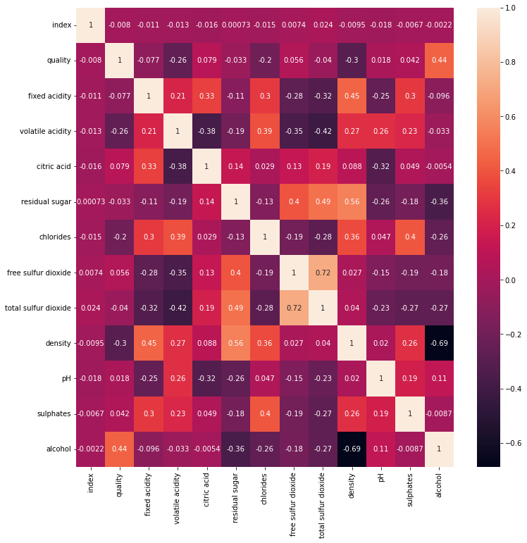
memory usage: 601.4+ KB# train의 변수 간 상관관계를 살펴봅니다.
plt.figure(figsize=(12,12))
sns.heatmap(data = train.corr(), annot=True)
<AxesSubplot:># train의 각 변수별 분포를 살펴봅니다.
plt.figure(figsize=(12,12))
for i in range(1,13):
plt.subplot(3,4,i)
sns.distplot(train.iloc[:,i])
plt.tight_layout()
plt.show()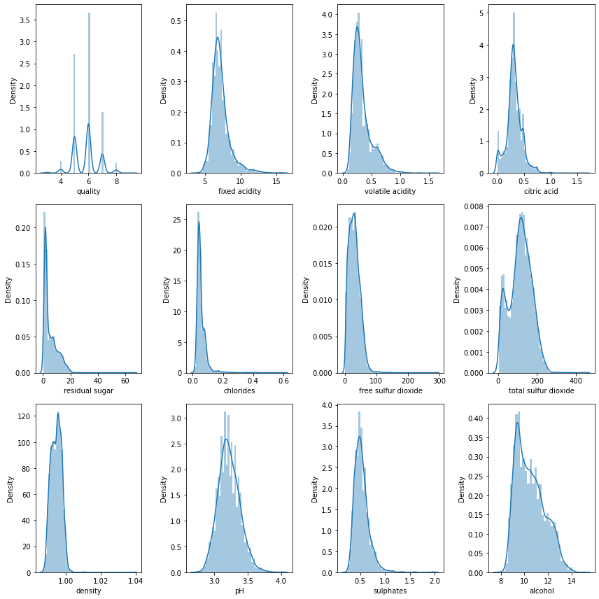
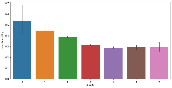
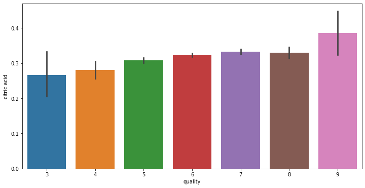
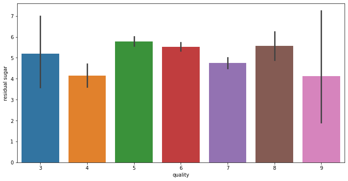
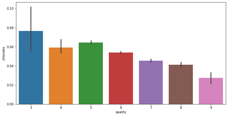
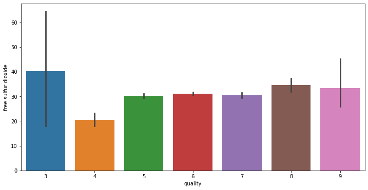
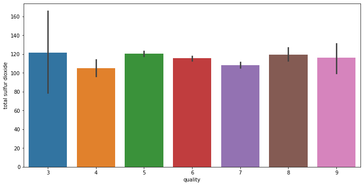
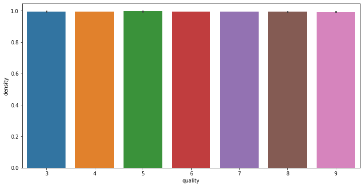
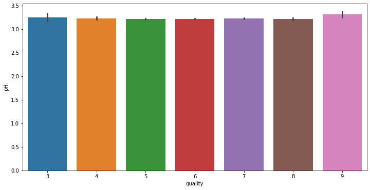
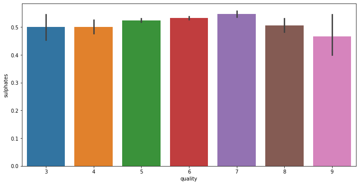
# train에서 각 변수와 quality 변수 사이 분포를 확인합니다.
for i in range(11):
    fig = plt.figure(figsize = (12,6))
    sns.barplot(x = 'quality', y = train.columns[i+2], data = train)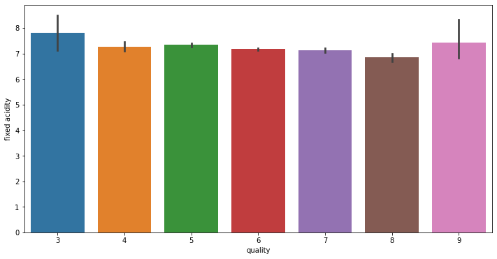

데이터 전처리
# type에는 white와 red 두 종류가 있습니다.
# 각각 0,1로 변환합니다.
from sklearn.preprocessing import LabelEncoder

enc = LabelEncoder()
enc.fit(train['type'])
train['type'] = enc.transform(train['type'])
test['type'] = enc.transform(test['type'])train.head()| index | quality | fixed acidity | volatile acidity | citric acid | residual sugar | chlorides | free sulfur dioxide | total sulfur dioxide | density | pH | sulphates | alcohol | type | |
|---|---|---|---|---|---|---|---|---|---|---|---|---|---|---|
| 0 | 0 | 5 | 5.6 | 0.695 | 0.06 | 6.8 | 0.042 | 9.0 | 84.0 | 0.99432 | 3.44 | 0.44 | 10.2 | 1 |
| 1 | 1 | 5 | 8.8 | 0.610 | 0.14 | 2.4 | 0.067 | 10.0 | 42.0 | 0.99690 | 3.19 | 0.59 | 9.5 | 0 |
| 2 | 2 | 5 | 7.9 | 0.210 | 0.39 | 2.0 | 0.057 | 21.0 | 138.0 | 0.99176 | 3.05 | 0.52 | 10.9 | 1 |
| 3 | 3 | 6 | 7.0 | 0.210 | 0.31 | 6.0 | 0.046 | 29.0 | 108.0 | 0.99390 | 3.26 | 0.50 | 10.8 | 1 |
| 4 | 4 | 6 | 7.8 | 0.400 | 0.26 | 9.5 | 0.059 | 32.0 | 178.0 | 0.99550 | 3.04 | 0.43 | 10.9 | 1 |
# 불필요한 변수 제거
X_train = train.drop(['index', 'quality'], axis = 1)
y_train = train['quality']
X_test = test.drop('index', axis = 1)
모델링 진행
from sklearn.ensemble import RandomForestClassifier
# 모델 선언
model = RandomForestClassifier()

#모델 학습
model.fit(X_train, y_train)RandomForestClassifier()# 학습된 모델로 test 데이터 예측
y_pred = model.predict(X_test)y_pred.shape(1000,)제출 파일 생성
submission = pd.read_csv('와인품질분류/data/sample_submission.csv')submission['quality'] = y_predsubmission| index | quality | |
|---|---|---|
| 0 | 0 | 5 |
| 1 | 1 | 6 |
| 2 | 2 | 6 |
| 3 | 3 | 5 |
| 4 | 4 | 6 |
| ... | ... | ... |
| 995 | 995 | 6 |
| 996 | 996 | 6 |
| 997 | 997 | 5 |
| 998 | 998 | 6 |
| 999 | 999 | 6 |
1000 rows × 2 columns
# csv 파일로 저장합니다.
submission.to_csv('미니프로젝트.csv', index=False)
배운걸 다 흡수하는 제로민