1. Reference Frames

Vector quantities can be expressed in different reference frames.

• Reference Frames

  • ECIF (Earth-Centred Inertial Frame)

    -	-
    x	fixed w.r.t stars
    y	fixed w.r.t stars
    z	true north

  • ECEF (Earth-Centred Earth-Fixed Frame)

    -	-
    x	prime meridian (on equator)
    y	Right-hand Rule
    z	true north

  • NED (North East Down)

    -	-
    x	true north
    y	true east
    z	down (along gravity)

  • ENU (East North Up)

    -	-
    x	true east
    y	true north
    z	up

  • Sensor & Vehicle

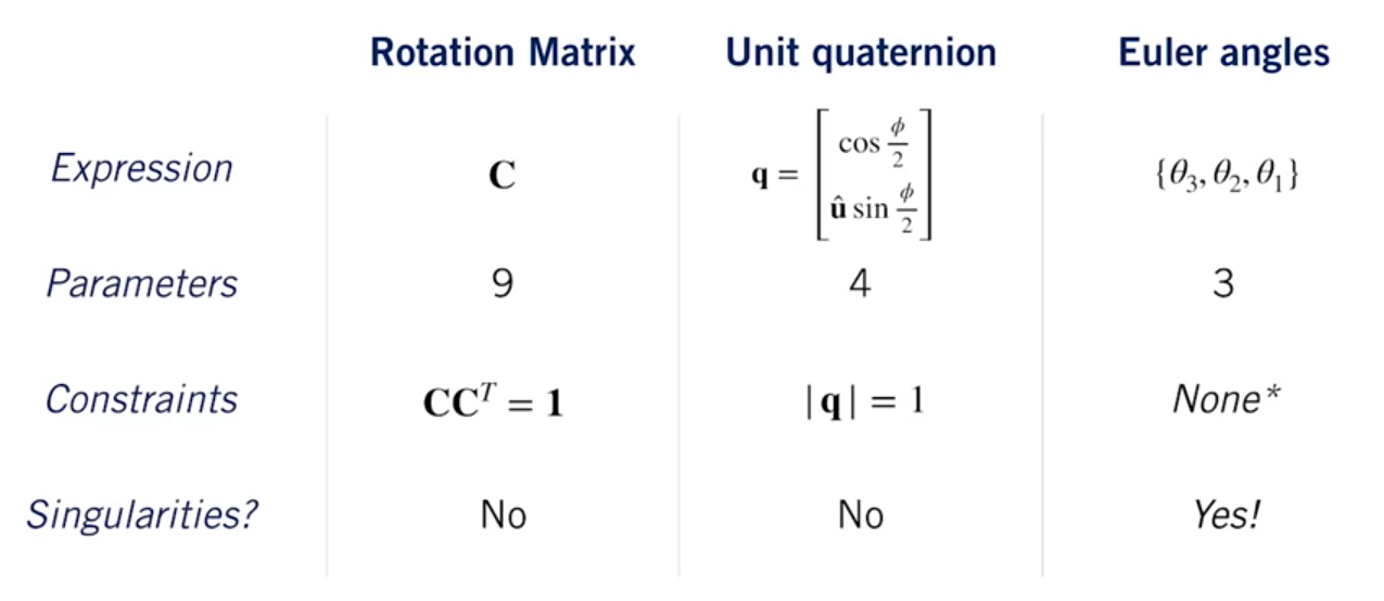
• Rotations can be parameterized by rotation matrices, quaternions or Euler angles.
  

---

2. IMU (Inertial Measurement Unit)

• An 6-DoF IMU is typically composed of

  • Gyroscopes
    measure angular rotation rates about three separate axes.
  • Accelerometers
    measure accelerations along three orthogonal axes.

• Measurement Model

  • Gyroscope

    $\omega(t) = \omega_s(t) + \mathbf{b}_{\text{gyro}}(t) + \mathbf{n}_{\text{gyro}}(t)$
    • $\omega_s(t)$: angular velocity of the sensor expressed in the sensor frame
    • $\mathbf{b}_{\text{gyro}}(t)$: slowly evolving bias
    • $\mathbf{n}_{\text{gyro}}(t)$: noise term

  • Accelerometer

    $a(t) = C_{sn}(t) (\ddot{\mathbf{r}}_n^{sn}(t) - \mathbf{g}_n) + \mathbf{b}_{\text{accel}}(t) + \mathbf{n}_{\text{accel}}(t)$
    • Instead of measuring body accelerations directly as we could do with rotational rates, we need to explicitly remove the effect of gravity using our fundamental equation for accelerometers in a gravity field.
    • $C_{sn}(t)$: orientation of the sensor (computed by integrating the rotational rates from the gyroscope)
    • $\mathbf{b}_{\text{accel}}(t)$: bias term
    • $\mathbf{n}_{\text{accel}}(t)$: noise term
    • $\mathbf{g}_n$: gravity in the navigation frame

• Since strapdown IMUs are tricky to calibrate and drift over time, we'll need another sensor to periodically correct our posed estimates.

---

3. GNSS (Global Navigation Satellite Systems)

• Computing Position

  • Each GPS satellite transmits a signal that encodes
    • its position
      (via accurate ephemeris information)
    • time of signal transmission
      (via onboard atomic clock)
  • To compute a GPS position fix in the Earth-centred frame, the receiver uses the speed of light to compute distances to each satellite based on time of signal arrvial.
  • At least four satellites are required to solve for 3D position, three if only 2D is required.

• Trilateration
  

  • different from Triangulation
  • For each satellite, we measure the pseudorange as follows:
    $\rho^{(i)} = c (T_r - t_s) = \sqrt{(\mathbf{p}^{(i)} - \mathbf{r})^T (\mathbf{p}^{(i)} - \mathbf{r})} + c \Delta t_r + c \Delta t_a^{(i)} + \eta^{(I)}$
    • $\mathbf{r}$: receiver (3D) position
    • $\mathbf{p}^{(i)}$: position of satellite $i$
    • $\Delta t_r$: receiver clock error
    • $\Delta t_a^{(i)}$: atmospheric propagation delay
    • $\eta$: measurement noise
    • $c$: speed of light
    • $t_s, t_r$: time sent, time received
  • By using at least 4 satellites, we can solve for:
    • $\mathbf{r}$ and $\Delta t_r$

• Error sources

  • Lonospheric delay (charged ions in the atmosphere)
  • Multipath effects (surrounding terrain or buildings)
  • Ephemeris & clock errors
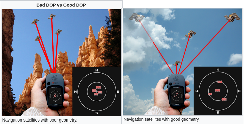
  • GDOP (Geometric Dilution of Precision)
    

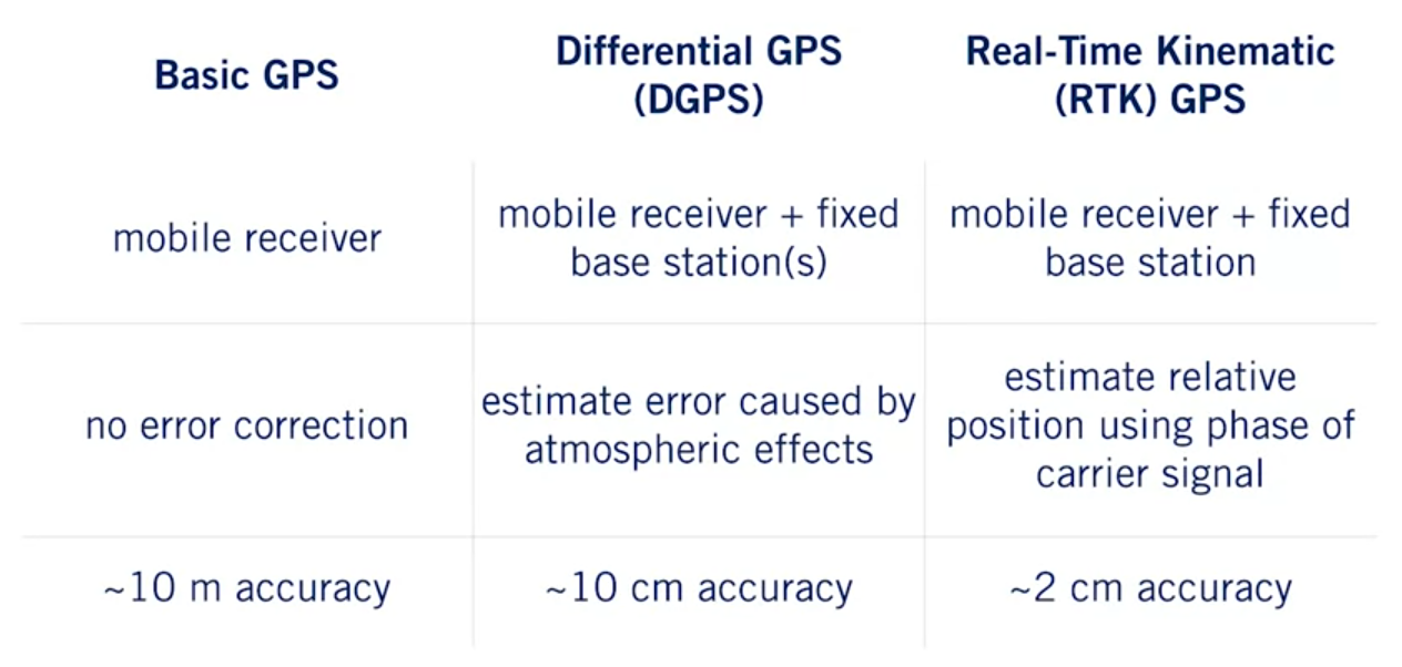
• How to improve accuracy
  

• Inertial sensors are useful for navigation but tend to drift, leading to increasing errors over time. On the other hand, GPS provides consistent positioning accuracy with bounded errors. A self-driving car using GPS will maintain reliable accuracy unless the GPS receiver fails or loses connection with at least four satellites.

---

4. LiDAR

• Measuring distance with Time-of-Flight

  $r = \frac{1}{2} c \cdot t$
  • $r$: Distance
  • $c$: Speed of light
  • $t$: Time elapsed (round-trip)

• Measurement Models for 3D LiDAR Sensors
  

• Measurement Noise

  • Sources
    • Uncertainty in determining the exact time of arrival of the reflected signal
    • Uncertainty in measuring the exact orientation of the mirror
    • Interaction with the target (surface absorption, specular reflection, etc.)
    • Variation of propagation speed (e.g. through materials)
  • Term
    $\mathbf{v} \sim \mathcal{N}(\mathbf{0}, \mathbf{R})$
    • Covariance: empirically determined or manually tuned

• Motion Distortion

  • For a vehicle which moves quickly, each point in a scan is taken from a slightly different place.

• Translation, Rotation and Scaling

  • Translation

    $\begin{bmatrix} X_{c2} \\ Y_{c2} \\ Z_{c2} \end{bmatrix} = \begin{bmatrix} X_{c1} \\ Y_{c1} \\ Z_{c1} \end{bmatrix} + \begin{bmatrix} t_{x} \\ t_{y} \\ t_{z} \end{bmatrix}$

  • Rotation

    $\begin{bmatrix} X_{c2} \\ Y_{c2} \\ Z_{c2} \end{bmatrix} = \mathbf{R} \begin{bmatrix} X_{c1} \\ Y_{c1} \\ Z_{c1} \end{bmatrix}$

  • Scaling

    $\begin{bmatrix} X_{c2} \\ Y_{c2} \\ Z_{c2} \end{bmatrix} = \mathbf{S} \begin{bmatrix} X_{c1} \\ Y_{c1} \\ Z_{c1} \end{bmatrix}$

• 3D Plane Fitting

  $\begin{aligned} e_j &= \hat{z}_j - z_j \\ &= (\hat{a} + \hat{b} x_j + \hat{c} y_j) - z_j \qquad j = 1, ..., n \end{aligned}$

• ICP Algorithm (Iterative Closest Point)

---

📙 강의

• University of Toronto - State Estimation and Localization for Self-Driving Cars